
Davide Pierangeli, Giulia Marcucci, Claudio Conti, "Photonic extreme learning machine by free-space optical propagation," Photonics Res. 9, 1446 (2021)
- Photonics Research
- Vol. 9, Issue 8, 1446 (2021)
Abstract
1. INTRODUCTION
Artificial neural networks excel in learning from data to perform classification, regression, and prediction tasks of vital importance [1]. As data information content increases, simulating these models becomes computationally expensive on conventional computers, making specialized signal processors crucial for intelligent systems. Training large networks is also costly in terms of energy consumption and carbon footprint [2]. Photonics provides a valuable alternative toward sustainable computing technologies. For this reason, machine learning through photonic components is gaining enormous interest [3]. In fact, many mathematical functions, which enable complex feature extraction from data, find a native implementation on optical platforms. Pioneering attempts using photosensitive masks [4] and volume holograms [5,6] have been recently developed into coherent optical neural networks that promise fast and energy-efficient optical computing [7–16]. These schemes exploit optical units such as nanophotonic circuits [7], on-chip frequency combs [14–16], and spatial light modulators to perform matrix multiplications in parallel [17] or to carry out convolutional layers [18–20]. Training consists in adjusting the optical response of each physical node [21], also by adopting external optical signals [22], which is demanding [23]. Moreover, photonic neural networks based on nanofabrication still have a considerable energy impact. A general and promising idea to overcome the issue is to adapt machine-learning paradigms and make them inclined to optical platforms. In this paper, we pursue this approach by constructing an easy-to-train optical architecture that requires only free-space optical propagation.
Photonic architectures that do not need control of the entire network are particularly attractive. A remarkable method for their design and training is reservoir computing [24–26], in which the nonlinear dynamics of a recurrent system processes data, and training occurs only on the readout layer. Optical reservoir computing has demonstrated striking performance on dynamical series prediction by using delay-based setups [27–30], laser networks [31], multimode waveguides [32], and random media [33]. Since several interesting complex systems can be exploited as physical reservoirs, the inverse approach is also appealing, i.e., the scheme can be trained for learning dynamical properties of the reservoir itself [34].
Extreme learning machines (ELMs) [35,36], or closely related schemes based on random neural networks [37,38], support vector machines [39] and kernel methods [40], are a powerful paradigm in which only a subset of connections is trained. ELMs perform comparably with basic deep and recurrent neural networks on the majority of learning tasks [36]. The basic mechanism is to use the network to establish a nonlinear mapping between the data set and a high-dimensional feature space, where a properly trained classifier performs the separation. Training occurs at the readout layer; however, at variance with reservoir computing, ELMs have no recurrences in the connection topology and do not possess dynamical memory. In optics, an interesting case of this general approach has been implemented by using speckle patterns emerging from multiple scattering [41] and multimode fibers [42] as a feature mapping. Although in principle many optical phenomena can form the building block of the architecture [43,44], the general potential of the ELM framework for photonic computing remains largely unexplored.
Sign up for Photonics Research TOC. Get the latest issue of Photonics Research delivered right to you!Sign up now
Here, we propose a photonic extreme learning machine (PELM) for performing classification and regression tasks using coherent light. We find that a minimal optical setting composed by an input element, which encodes embedded input data into the optical field, a wave layer, corresponding to propagation in free space, and a nonlinear detector, enables simple and efficient learning. The encoding method plays a crucial role in determining the learning ability of the machine. The architecture is experimentally implemented via phase modulation of a visible laser beam by a spatial light modulator (SLM). We benchmark the realized device on problems of different classes, achieving performance comparable with digital ELMs. These include a classification accuracy exceeding 92% on the well-known MNIST database, which overcomes fabricated diffractive neural networks [8]; further, it is comparable with convolutional artificial networks that employ photonic accelerators [15,16,19]. Given the massive parallelism provided by spatial optics and the ease of training, our approach is ideal for big data, i.e., extensive data sets with large dimension samples. Our PELM is intrinsically stable and adaptable over time, as it does not require engineered or sensitive components. It can potentially operate in dynamic environments as an intelligent device performing on-the-fly optical signal processing.
2. PELM ARCHITECTURE
An ELM is a feed-forward neural network in which a set of input signals is connected to at least one output node by a large structure of generalized artificial neurons [35]. An outline of the architecture is illustrated in Fig. 1(a). The hidden neurons form the computing reservoir. Unlike for neurons in a deep neural network, they do not require any training, and their individual responses can be unknown to the user [36]. Given an input data set with
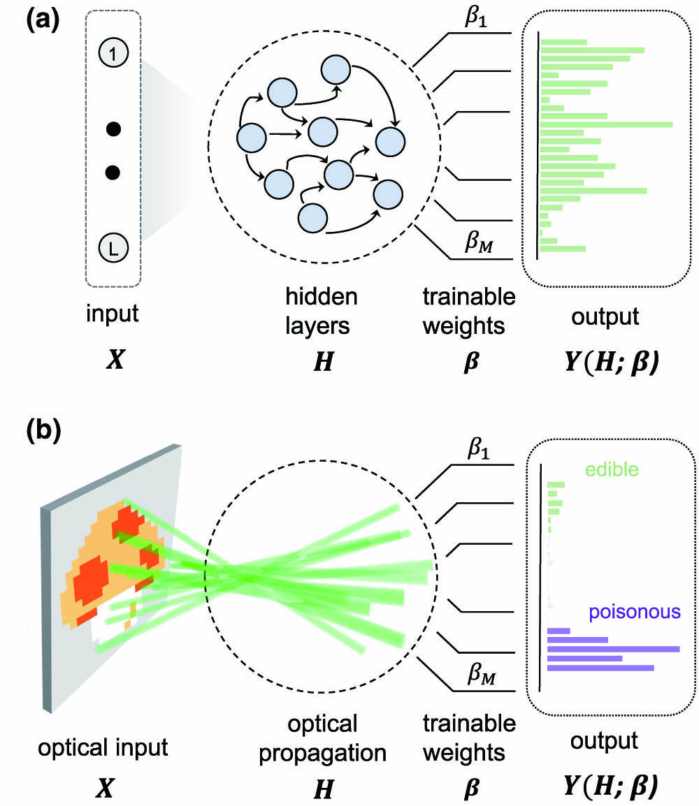
Figure 1.Schematic architecture of the photonic extreme learning machine (PELM). (a) General ELM scheme with the input data set
We transfer the ELM principle into the optical domain by considering the three-layer structure illustrated in Fig. 1(b). In the encoding layer, the input vectors
In the PELM architecture, each operation is defined by the corresponding optical elements. Therefore, Eq. (2) can represent the feature space of different optical settings. For instance, in the optical classifier demonstrated by Saade
We first validate the free-space PELM architecture and assess the condition for learning via numerical simulations. We consider digit recognition and train our classifier on the MNIST handwritten digit database. Figure 2 reports the learning properties for two representative phase-encoding methods: (i) noise embedding and (ii) Fourier embedding. In (i),
![]()
Figure 2.Learning ability of the PELM architecture. The optical computing scheme is evaluated on the MNIST data set by varying the encoding properties and feature space. (a) Input digit and 2D phase mask showing its encoding by noise embedding: the input signal overlaps with a disordered matrix. PELM training and testing error for noise embedding when varying the (b) noise amplitude and (c) its correlation length, for
Another key hyperparameter of the scheme is the number of features (channels)
3. EXPERIMENTAL DEVICE
The experimental setup for the free-space photonic extreme learning machine is illustrated in Fig. 3(a) and detailed in Appendix B. A phase-only SLM encodes both the input data set and the embedding matrix on the phase spatial profile of the laser beam. In practice, distinct attributes of a data set are arranged in separate blocks, a data sample corresponds to a set of phase values on these blocks, and a preselected phase mask is superimposed [inset in Fig. 3(a)]. Phase information self-mixes during light propagation, a linear process that corresponds to the matrix multiplication in Eq. (2). The far field is detected on a camera that performs the nonlinear activation function. As shown in Fig. 3(b), the resulting acquired image is a saturated function of the optical amplitude in the lens focal plane. From this data matrix, we extract the
![]()
Figure 3.Experimental implementation. (a) Sketch of the optical setup. A phase-only spatial light modulator (SLM) encodes data on the wavefront of a 532 nm continuous-wave laser. The far field in the lens focal plane is imaged on a camera. Insets show a false-color embedding matrix and training data encoded as phase blocks, respectively. (b) Detected spatial intensity distribution for a given input sample. White-colored areas reveal camera saturation in high-intensity regions, which provides the network nonlinear function. Pink boxes show some of the
We test the optical device on various computing tasks and data sets. The aim is to point out that, when the PELM is fully effective on a given task, it can be also easily and rapidly retrained for a different application. The main results are summarized in Fig. 4 and demonstrate the learning capability of the optical device. We first use the MNIST data set to prove classification on a large-scale multiclass problem. When trained using
![]()
Figure 4.Experimental performance of the PELM on classification and regression tasks. Confusion matrices on the MNIST data set for a free-space PELM, which makes use of (a) Fourier and (b) random embedding (92.18% and 92.06% accuracy,
By only updating the input training set and the output weights, the PELM can be quickly reconfigured for classifying different objects. We consider a binary class problem, i.e., the mushroom task, where the goal is to separate poisonous from edible mushrooms from a series of features (see Appendix C for details). Figure 4(c) shows that, on this data set, we achieve 95.4% accuracy, using
A key point of the PELM architecture is a testing error that rapidly converges to its optimal value as the feature space dimension increases. Experimental results demonstrating this property are shown in Figs. 4(e) and 4(f), respectively, for the MNIST and abalone data set. Good classification/regression performance is maintained even for a very small number of trained channels, if compared with the data set size. For instance, useful abalone predictions can be obtained with only
It is worth noting that the device does not need training at each use. Once we learn a given data set, we store the corresponding output weights and program a different problem; then, we are able to accomplish any of the posed tasks on-demand. The diverse classification and regression instances in Fig. 4 can be tested without any sequential order, simply specifying the type of task they belong to.
4. DISCUSSION
A. Improving the Photonic Hardware
The limit provided by training errors in Figs. 4(e) and 4(f) allows us to identify the various factors toward improving the computational resolution of the optical machine. We ascribe residual errors to practical nonidealities of the device. The finite precision of both encoding and readout, including noise in optical intensities, introduces errors that are absent in the digital implementation [48]. Considering a camera precision of 8 bit in the numerical model, we find a relevant decrease of the maximum accuracy. This indicates that improved performance is attainable by fine-tuning the optical components. Flickering effects of the phase modulator, which give a tiny but variable inaccuracy each time the machine is interrogated, are identified as another relevant source of error. Moreover, optical and mechanical fluctuations of the tabletop optical line during training can result in further inconsistencies. These fluctuations can be compensated in future experiments using incremental learning [36], a refined technique that allows us to adaptively adjust the weights while training is ongoing. Training by use of sparse regression methods may be also useful when dealing with larger data sets.
B. Comparison with Digital Kernel Methods
The learning principle of the PELM lies on the basis of various kernel methods [49]. In kernel classification, mapping of the input data to the high-dimensional feature space is not explicit, and correlations between samples are evaluated through a kernel function over the input space. Such a kernel
C. Application Potentials
Besides computing effectiveness comparable with its digital counterpart, the PELM hardware offers several advantages that are promising for fast processing of big data, especially for inputs that naturally present themselves as optical signals. In fact, unlike deep optical neural networks [51,52], training is simple and scales favorably with the data set size. It can also be performed online with affordable computational resources. Once trained, forward information propagates optically in a fully passive way and in free space. This can provide a key advantage with respect to ELM algorithms and kernel methods both in terms of scalability and latency. In fact, the matrix multiplication in Eq. (2), which maps input data to the feature space, on a digital computer requires a time and memory consumption that grows quadratically with the data dimension
The absence of any optical element or medium along the network path, which differentiates our scheme from all other optical neuromorphic devices previously realized, is a valuable aspect for various reasons. The tiny optical absorption and scattering of light in air imply that our scheme needs low-power optical sources (
In view of edge-computing applications, the PELM can be further adapted toward ease of use and energy efficiency. In fact, using optical signals from the environment as input data, the encoding operation performed by the SLM is reduced to the sole embedding. This operation can be integrated directly into optical propagation, removing the need for a phase modulator. For example, we can divide the coherent input field and recombine it after a digital micromirror device (DMD) has performed the embedding. The intensity extracted from a selected plane along the optical path gives the output matrix, which can be enriched with phase and spectral information. Similar schemes promise a miniaturization of our free-space device and its operation as a fast and stable optical processor.
5. CONCLUSION
Nowadays, artificial intelligence is permeating the field of photonics [55,56] and viceversa [57]. Optical platforms are enabling computing functionalities with unique features, ranging from photonic Ising machines for complex optimization problems [58–65] to optical devices for cryptography [66]. We have realized a novel photonic neuromorphic computing device that is able to perform classification and feature extraction only by exploiting optical propagation in free space. Our results demonstrate that fabricated optical networks, or complex physical processes and materials, are not mandatory ingredients for performing effective machine learning on a optical setup. All the essential factors for learning can be included in optical propagation via encoding and decoding methods. On this principle, we demonstrated a photonic extreme-learning machine that, given its unique adaptability and intrinsic stability, is attractive for future processing of optical data in real-time and dynamic conditions. More generally, our approach envisions the exceptional possibility of harnessing any wave system as an intelligent device that learns from data, in photonics, and far beyond.
Acknowledgment
Acknowledgment. We thank MD Deen Islam and V. H. Santos for technical support in the laboratory.
APPENDIX A: NETWORK DETAILS
The basic ELM structure is a single-layer feedforward neural network in which hidden nodes are not tuned [
In the case of a single-output node performing binary classification [as for the problem in Fig.
We consider phase encoding of the input data in all the presented results (phase-only light modulation). The embedding matrix
APPENDIX B: EXPERIMENTAL SETUP AND DEVICE TRAINING
A continuous-wave laser beam with wavelength
Training is performed by loading one by one the
APPENDIX C: DATA SETS FOR CLASSIFICATION AND REGRESSION
Recognition of handwritten digits is tested on the MNIST data set, a standard benchmark for multiclass classification. The data set, which includes 10 classes, consists of 60,000 training samples (
The mushroom (https://archive.ics.uci.edu/ml/datasets/Mushroom) is a binary class data set with relatively large size and low dimension. It includes 8124 samples with
The abalone data set (https://archive.ics.uci.edu/ml/datasets/Abalone) is one of the mostly used benchmarks for machine learning and concerns the identification of sea snails in terms of age and physical parameters. Each training point has
References
[1] S. Haykin. Neural Networks and Learning Machines(2008).
[2] E. Strubell, A. Ganesh, A. McCallum. Energy and policy considerations for deep learning in NLP(2019).
[3] G. Wetzstein, A. Ozcan, S. Gigan, S. Fan, D. Englund, M. Soljačić, C. Denz, D. A. B. Miller, D. Psaltis. Inference in artificial intelligence with deep optics and photonics. Nature, 588, 39-47(2020).
[4] N. H. Farhat, D. Psaltis, A. Prata, E. Paek. Optical implementation of the Hopfield model. Appl. Opt., 24, 1469-1475(1985).
[5] D. Psaltis, D. Brady, K. Wagner. Adaptive optical networks using photorefractive crystals. Appl. Opt., 27, 1752-1759(1988).
[6] C. Denz. Optical Neural Networks(1998).
[7] Y. Shen, N. C. Harris, S. Skirlo, M. Prabhu, T. Baehr-Jones, M. Hochberg, X. Sun, S. Zhao, H. Larochelle, D. Englund, M. Soljacic. Deep learning with coherent nanophotonic circuits. Nat. Photonics, 11, 441-446(2017).
[8] X. Lin, Y. Rivenson, N. T. Yardimci, M. Veli, Y. Luo, M. Jarrahi, A. Ozcan. All-optical machine learning using diffractive deep neural networks. Science, 361, 1004-1008(2018).
[9] N. M. Estakhri, B. Edwards, N. Engheta. Inverse-designed metastructures that solve equations. Science, 363, 1333-1338(2019).
[10] J. Bueno, S. Maktoobi, L. Froehly, I. Fischer, M. Jacquot, L. Larger, D. Brunner. Reinforcement learning in a large-scale photonic recurrent neural network. Optica, 5, 756-760(2018).
[11] Y. Zuo, B. Li, Y. Zhao, Y. Jiang, Y. C. Chen, P. Chen, G. B. Jo, J. Liu, S. Du. All-optical neural network with nonlinear activation functions. Optica, 6, 1132-1137(2019).
[12] A. N. Tait, T. F. de Lima, E. Zhou, A. X. Wu, M.-A. Nahmias, B. J. Shastri, P. R. Prucnal. Neuromorphic photonic networks using silicon photonic weight banks. Sci. Rep., 7, 7430(2017).
[13] J. Feldmann, N. Youngblood, C. D. Wright, H. Bhaskaran, W. H. P. Pernice. All-optical spiking neurosynaptic networks with self-learning capabilities. Nature, 569, 208-214(2019).
[14] J. Feldmann, N. Youngblood, M. Karpov, H. Gehring, X. Li, M. Stappers, M. Le Gallo, X. Fu, A. Lukashchuk, A. S. Raja, J. Liu, C. D. Wright, A. Sebastian, T. J. Kippenberg, W. H. P. Pernice, H. Bhaskaran. Parallel convolutional processing using an integrated photonic tensor core. Nature, 589, 52-58(2021).
[15] X. Xu, M. Tan, B. Corcoran, J. Wu, A. Boes, T. G. Nguyen, S. T. Chu, B. E. Little, D. G. Hicks, R. Morandotti, A. Mitchell, D. J. Moss. 11 TOPS photonic convolutional accelerator for optical neural networks. Nature, 589, 44-51(2021).
[16] X. Xu, M. Tan, B. Corcoran, J. Wu, T. G. Nguyen, A. Boes, S. T. Chu, B. E. Little, R. Morandotti, A. Mitchell, D. G. Hicks, D. J. Moss. Photonic perceptron based on a Kerr microcomb for high-speed, scalable, optical neural networks. Laser Photon. Rev., 14, 2000070(2020).
[17] J. Spall, X. Guo, T. D. Barrett, A. I. Lvovsky. Fully reconfigurable coherent optical vector-matrix multiplication. Opt. Lett., 45, 5752-5755(2020).
[18] J. Chang, V. Sitzmann, X. Dun, W. Heidrich, G. Wetzstein. Hybrid optical-electronic convolutional neural networks with optimized diffractive optics for image classification. Sci. Rep., 8, 12324(2018).
[19] M. Miscuglio, Z. Hu, S. Li, J. George, R. Capanna, P. M. Bardet, P. Gupta, V. J. Sorger. Massively parallel amplitude-only Fourier neural network. Optica, 7, 1812-1819(2020).
[20] C. Wu, H. Yu, S. Lee, R. Peng, I. Takeuchi, M. Li. Programmable phase-change metasurfaces on waveguides for multimode photonic convolutional neural network. Nat. Commun., 12, 96(2021).
[21] T. W. Hughes, I. A. Williamson, M. Minkov, S. Fan. Wave physics as an analog recurrent neural network. Sci. Adv., 5, eaay6946(2019).
[22] R. Hamerly, L. Bernstein, A. Sludds, M. Soljačić, D. Englund. Large-scale optical neural networks based on photoelectric multiplication. Phys. Rev. X, 9, 021032(2019).
[23] T. W. Hughes, M. Minkov, Y. Shi, S. Fan. Training of photonic neural networks through
[24] M. Lukosevicius, H. Jaeger. Reservoir computing approaches to recurrent neural network training. Comput. Sci. Rev., 3, 127-149(2009).
[25] C. Gallicchio, A. Micheli, L. Pedrelli. Deep reservoir computing: a critical experimental analysis. Neurocomputing, 268, 87-99(2017).
[26] G. Neofotistos, M. Mattheakis, G. D. Barmparis, J. Hizanidis, G. P. Tsironis, E. Kaxiras. Machine learning with observers predicts complex spatiotemporal behavior. Front. Phys., 7, 24(2019).
[27] D. Brunner, M. C. Soriano, C. Mirasso, I. Fischer. Parallel photonic information processing at gigabyte per second data rates using transient states. Nat. Commun., 4, 1364(2013).
[28] Q. Vinckier, F. Duport, A. Smerieri, K. Vandoorne, P. Bienstman, M. Haelterman, S. Massar. High-performance photonic reservoir computer based on a coherently driven passive cavity. Optica, 2, 438-446(2015).
[29] L. Larger, A. Baylón-Fuentes, R. Martinenghi, V. S. Udaltsov, Y. K. Chembo, M. Jacquot. High-speed photonic reservoir computing using a time-delay based architecture: million words per second classification. Phys. Rev. X, 7, 011015(2017).
[30] P. Antonik, N. Marsal, D. Brunner, D. Rontani. Human action recognition with a large-scale brain-inspired photonic computer. Nat. Mach. Intell., 1, 530-537(2019).
[31] A. Röhm, L. Jaurigue, K. Lüdge. Reservoir computing using laser networks. IEEE J. Sel. Top. Quantum Electron., 26, 7700108(2020).
[32] U. Paudel, M. Luengo-Kovac, J. Pilawa, T. J. Shaw, G. C. Valley. Classification of time-domain waveforms using a speckle-based optical reservoir computer. Opt. Express, 28, 1225-1237(2020).
[33] M. Rafayelyan, J. Dong, Y. Tan, F. Krzakala, S. Gigan. Large-scale optical reservoir computing for spatiotemporal chaotic systems prediction. Phys. Rev. X, 10, 041037(2020).
[34] D. Pierangeli, V. Palmieri, G. Marcucci, C. Moriconi, G. Perini, M. De Spirito, M. Papi, C. Conti. Living optical random neural network with three dimensional tumor spheroids for cancer morphodynamics. Commun. Phys., 3, 160(2020).
[35] G. B. Huang, Q. Y. Zhu, C. K. Siew. Extreme learning machine: theory and applications. Neurocomputing, 70, 489-501(2006).
[36] G. B. Huang, H. Zhou, X. Ding, R. Zhang. Extreme learning machine for regression and multiclass classification. IEEE Trans. Syst., Man, Cybern. B, Cybern., 42, 513-529(2012).
[37] W. F. Schmidt, M. A. Kraaijveld, R. P. Duin. Feed forward neural networks with random weights. International Conference on Pattern Recognition(1992).
[38] Y. H. Pao, G. H. Park, D. J. Sobajic. Learning and generalization characteristics of the random vector functional-link net. Neurocomputing, 6, 163-180(1994).
[39] J. A. K. Suykens, J. Vandewalle. Least squares support vector machine classifiers. Neural Process. Lett., 9, 293-300(1999).
[40] S. An, W. Liu, S. Venkatesh. Face recognition using kernel ridge regression. IEEE Computer Society Conference on Computer Vision and Pattern Recognition, 1-7(2007).
[41] A. Saade, F. Caltagirone, I. Carron, L. Daudet, A. Dremeau, S. Gigan, F. Krzakala. Random projections through multiple optical scattering: approximating kernels at the speed of light. IEEE International Conference on Acoustics, Speech and Signal Processing (ICASSP), 6215-6219(2016).
[42] S. Sunada, K. Kanno, A. Uchida. Using multidimensional speckle dynamics for high-speed, large-scale, parallel photonic computing. Opt. Express, 28, 30349-30361(2020).
[43] G. Marcucci, D. Pierangeli, C. Conti. Theory of neuromorphic computing by waves: machine learning by rogue waves, dispersive shocks, and solitons. Phys. Rev. Lett., 125, 093901(2020).
[44] U. Tegin, M. Yildirim, I. Oguz, C. Moser, D. Psaltis. Scalable optical learning operator(2020).
[45] H. Zhang, M. Gu, X. D. Jiang, J. Thompson, H. Cai, S. Paesani, R. Santagati, A. Laing, Y. Zhang, M. H. Yung, Y. Z. Shi, F. K. Muhammad, G. Q. Lo, X. S. Luo, B. Dong, D. L. Kwong, L. C. Kwek, A. Q. Liu. An optical neural chip for implementing complex-valued neural network. Nat. Commun., 12, 457(2021).
[46] J. W. Goodman. Introduction to Fourier Optics(2005).
[47] L. C. C. Kasun, H. Zhou, G. B. Huang, C. M. Vong. Representational learning with extreme learning machine for big data. IEEE Intell. Syst., 28, 31-34(2013).
[48] D. Pierangeli, M. Rafayelyan, C. Conti, S. Gigan. Scalable spin-glass optical simulator. Phys. Rev. Appl., 15, 034087(2021).
[49] J. Shawe-Taylor, N. Cristianini. Kernel Methods for Pattern Analysis(2004).
[50] Y. Lecun, L. Bottou, Y. Bengio, P. Haffner. Gradient-based learning applied to document recognition. Proc. IEEE, 86, 2278-2324(1998).
[51] T. Yan, J. Wu, T. Zhou, H. Xie, F. Xu, J. Fan, L. Fang, X. Lin, Q. Dai. Fourier-space diffractive deep neural network. Phys. Rev. Lett., 123, 023901(2019).
[52] Y. Luo, D. Mengu, N. T. Yardimci, Y. Rivenson, M. Veli, M. Jarrahi, A. Ozcan. Design of task-specific optical systems using broadband diffractive neural networks. Light Sci. Appl., 8, 112(2019).
[53] O. Tzang, E. Niv, S. Singh, S. Labouesse, G. Myatt, R. Piestun. Wavefront shaping in complex media with a 350 kHz modulator via a 1D-to-2D transform. Nat. Photonics, 13, 788-793(2019).
[54] B. Braverman, A. Skerjanc, N. Sullivan, R. W. Boyd. Fast generation and detection of spatial modes of light using an acousto-optic modulator. Opt. Express, 28, 29112-29121(2020).
[55] D. Piccinotti, K. F. MacDonald, S. Gregory, I. Youngs, N. I. Zheludev. Artificial intelligence for photonics and photonic materials. Rep. Prog. Phys., 84, 012401(2021).
[56] G. Genty, L. Salmela, J. M. Dudley, D. Brunner, A. Kokhanovskiy, S. Kobtsev, S. K. Turitsyn. Machine learning and applications in ultrafast photonics. Nat. Photonics, 15, 91-101(2020).
[57] S. H. Rudy, S. L. Brunton, J. L. Proctor, J. N. Kutz. Data-driven discovery of partial differential equations. Sci. Adv., 3, e1602614(2017).
[58] P. L. McMahon, A. Marandi, Y. Haribara, R. Hamerly, C. Langrock, S. Tamate, T. Inagaki, H. Takesue, S. Utsunomiya, K. Aihara, R. L. Byer, M. M. Fejer, H. Mabuchi, Y. Yamamoto. A fully-programmable 100-spin coherent Ising machine with all-to-all connections. Science, 354, 614-617(2016).
[59] T. Inagaki, Y. Haribara, K. Igarashi, T. Sonobe, S. Tamate, T. Honjo, A. Marandi, P. L. McMahon, T. Umeki, K. Enbutsu, O. Tadanaga, H. Takenouchi, K. Aihara, K.-I. Kawarabayashi, K. Inoue, S. Utsunomiya, H. Takesue. A coherent Ising machine for 2000-node optimization problems. Science, 354, 603-606(2016).
[60] F. Böhm, G. Verschaffelt, G. Van der Sande. A poor—coherent Ising machine based on opto-electronic feedback systems for solving optimization problems. Nat. Commun., 10, 3538(2019).
[61] D. Pierangeli, G. Marcucci, C. Conti. Large-scale photonic Ising machine by spatial light modulation. Phys. Rev. Lett., 122, 213902(2019).
[62] D. Pierangeli, G. Marcucci, C. Conti. Adiabatic evolution on a spatial-photonic Ising machine. Optica, 7, 1535-1543(2020).
[63] M. Prabhu, C. Roques-Carmes, Y. Shen, N. Harris, L. Jing, J. Carolan, R. Hamerly, T. Baehr-Jones, M. Hochberg, V. Čeperić, J. D. Joannopoulos, D. R. Englund, M. Soljačić. Accelerating recurrent Ising machines in photonic integrated circuits. Optica, 7, 551-558(2020).
[64] K. P. Kalinin, A. Amo, J. Bloch, N. G. Berloff. Polaritonic XY-Ising machine. Nanophotonics, 9, 4127-4138(2020).
[65] Y. Okawachi, M. Yu, J. K. Jang, X. Ji, Y. Zhao, B. Y. Kim, M. Lipson, A. L. Gaeta. Demonstration of chip-based coupled degenerate optical parametric oscillators for realizing a nanophotonic spin-glass. Nat. Commun., 11, 4119(2020).
[66] A. Di Falco, V. Mazzone, A. Cruz, A. Fratalocchi. Perfect secrecy cryptography via mixing of chaotic waves in irreversible time-varying silicon chips. Nat. Commun., 10, 5827(2019).


Set citation alerts for the article
Please enter your email address

© Copyright 2018-2021 | Chinese Laser Press. All Rights Reserved 沪ICP备15018463号-20