Fig. 1. Phase unwrapping in OI,¹ MRI,² FPP,⁴ and InSAR.⁶

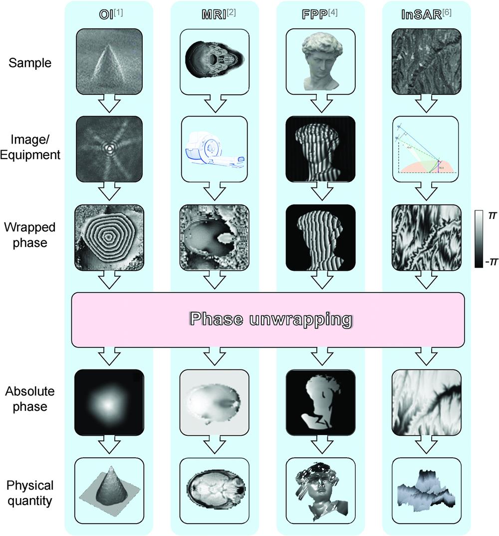
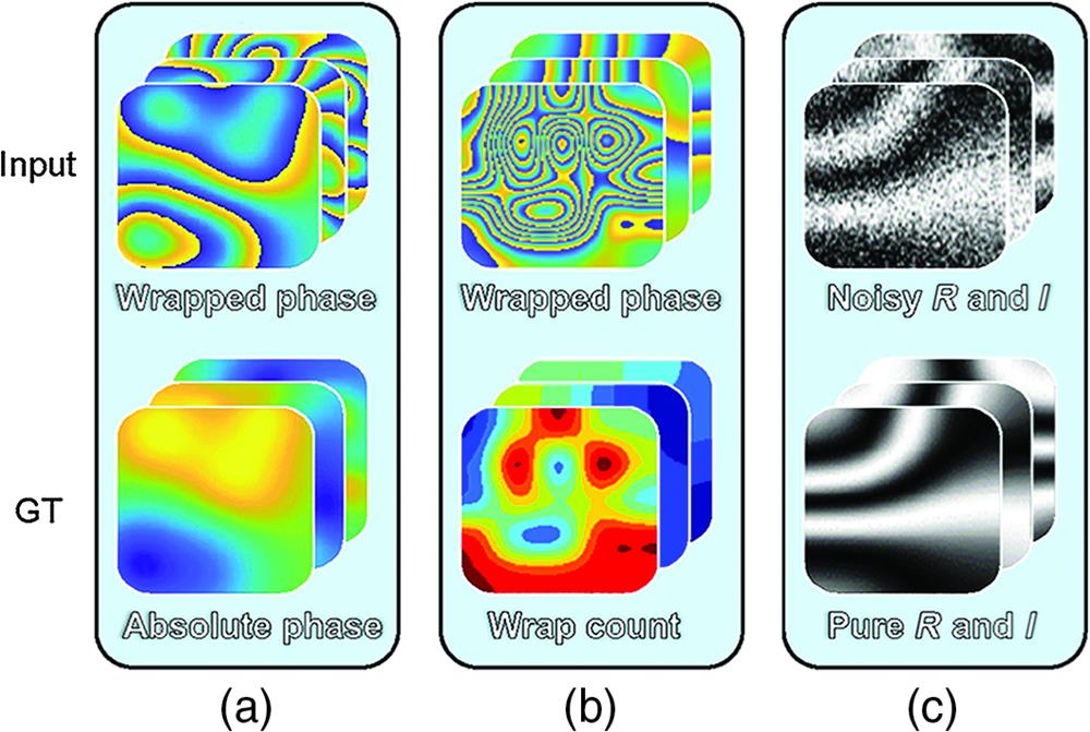
Fig. 2. Datasets of the deep-learning-involved phase unwrapping methods, for (a) dRG, (b) dWC, and (c) dDN. “$R$” and “$I$” represent the real and imaginary parts of CAF, respectively.

Fig. 3. Overall process of deep-learning-involved phase unwrapping methods.

Fig. 4. Illustration of the dRG method.

Fig. 5. Illustration of the dWC method.

Fig. 6. Illustration of the dDN method.

Fig. 7. An example of the RME method.

Fig. 8. An example of the GFS method.

Fig. 9. Entropy histogram of absolute phases from the D_RME, D_GFS, and D_ZPS.

Fig. 10. SAGD maps of different datasets. Red arrows and circles indicate low and high SAGD values, respectively.

Fig. 11. Mean error maps for each network. Red circles indicate high mean error value.

Fig. 12. (a) SAGD maps for D_RME and D_RME1, (b) mean error maps for RME-Net and RME1-Net. Red arrows indicate low SAGD value. Red circles indicate high mean error value and orange circles indicate the comparison part.

Fig. 13. Partial display of results from RME1-Net. “Max”, “Med,” and “Min” represent specific results with maximal, median, and minimal ${\mathrm{RMSE}}_{\mathrm{m}}$, respectively. “-C” represents the congruence results.

Fig. 14. Results for the (a) dRG-I and (b) dWC-I in the ideal case. “Max,” “Med,” and “Min” represent specific results with maximal, median, and minimal ${\mathrm{RMSE}}_{\mathrm{m}}$, respectively. “-C” represents the congruence results.

Fig. 15. ${\mathrm{RMSE}}_{\mathrm{m}}$ of the deep-learning-involved methods for absolute phase in different heights.

Fig. 16. Results for (a) dRG-N, (b) dWC-N, and (c) dDN-N in the noisy case. “GT” represents the pure GT (pure absolute phase), while “GT1” represents the noisy GT (noisy absolute phase). “Max,” “Med,” and “Min” represent specific results with maximal, median, and minimal ${\mathrm{RMSE}}_{\mathrm{m}}$, respectively. “-C” represents the congruence results.

Fig. 17. Results in different noise levels. Solid and dashed lines represent the deep-learning-involved and traditional methods, respectively.

Fig. 18. Results for (a) dRG-I, (b) dWC-I, (c) dRG-D, (d) dWC-D, (e) line-scanning, (f) LS, and (g) QG methods in the discontinuous case. “Max,” “Med,” and “Min” represent specific results with maximal, median, and minimal ${\mathrm{RMSE}}_{\mathrm{m}}$, respectively. “-C” represents the congruence results. The last columns of each result are discontinuous maps, where 1 (white) represents the position of the discontinuous pixels.

Fig. 19. Results for (a) dRG-A, (b) dWC-A, (c) line-scanning, (d) LS, and (e) QG methods in the aliasing case. “Max,” “Med,” and “Min” represent specific results with maximal, median, and minimal ${\mathrm{RMSE}}_{\mathrm{m}}$, respectively. “-C” represents the congruence results. The last columns of each result are aliasing maps, where 1 (white) represents the position of the aliasing pixels.

Fig. 20. Results for (a) dRG-M, (b) dWC-M, (c) line-scanning, (d) LS, and (e) QG methods in the mixed case. “Max,” “Med,” and “Min” represent specific results with maximal, median, and minimal ${\mathrm{RMSE}}_{\mathrm{m}}$, respectively. “$-\mathrm{C}$” represents the congruence results. The last columns of each result are aliasing or discontinuous maps (called “$\text{A}$ and $\text{D}$”), where 1 (white) represents the position of the aliasing or discontinuous pixels.

Fig. 21. Schematic diagram of pretraining and retraining.

Fig. 22. Loss plot of pretrained and initialized networks.

Table 1. Summary of deep-learning-involved phase unwrapping methods. “—” indicates “not available.”

Table 2. Summary of datasets. “—” indicates “not available.”

Table 3. RMSEm, RMSEsd, and PFS of phase unwrapping results of RME-Net, GFS-Net, and ZPS-Net.

Table 4. Summary of networks and corresponding datasets. The form of the dataset is {Input, GT}. The last letter of the network name is the case (“I” for ideal, “N” for noisy, “D” for discontinuous, “A” for aliasing, and “M” for mixed).

Table 5. RMSEm, RMSEsd, PFS, and PIP of the deep-learning-involved methods in the ideal case. “-C” represents the congruence results.

Table 6. RMSEm, RMSEsd, PFS, and PIP of the deep-learning-involved methods in the noisy case. “GT” represents the pure GT (pure absolute phase), while “GT1” represents the noisy GT (noisy absolute phase). “-C” represents the congruence results.

Table 7. RMSEm, RMSEsd, PFS, and PIP of the deep-learning-involved and traditional methods in the discontinuous case. “-C” represents the congruence results.

Table 8. RMSEm, RMSEsd, PFS, and PIP of the deep-learning-involved and traditional methods in the aliasing case. “-C” represents the congruence results.

Table 9. RMSEm, RMSEsd, PFS, and PIP of the deep-learning-involved and traditional methods in the mixed case. “-C” represents the congruence results.

Table 10. Performance statistics in the ideal, noisy, discontinuous, and aliasing cases. “✓” represents “capable.” “✓✓” represents “best and recommended.” “✗” represents “incapable.” “—” indicates “not applicable.”