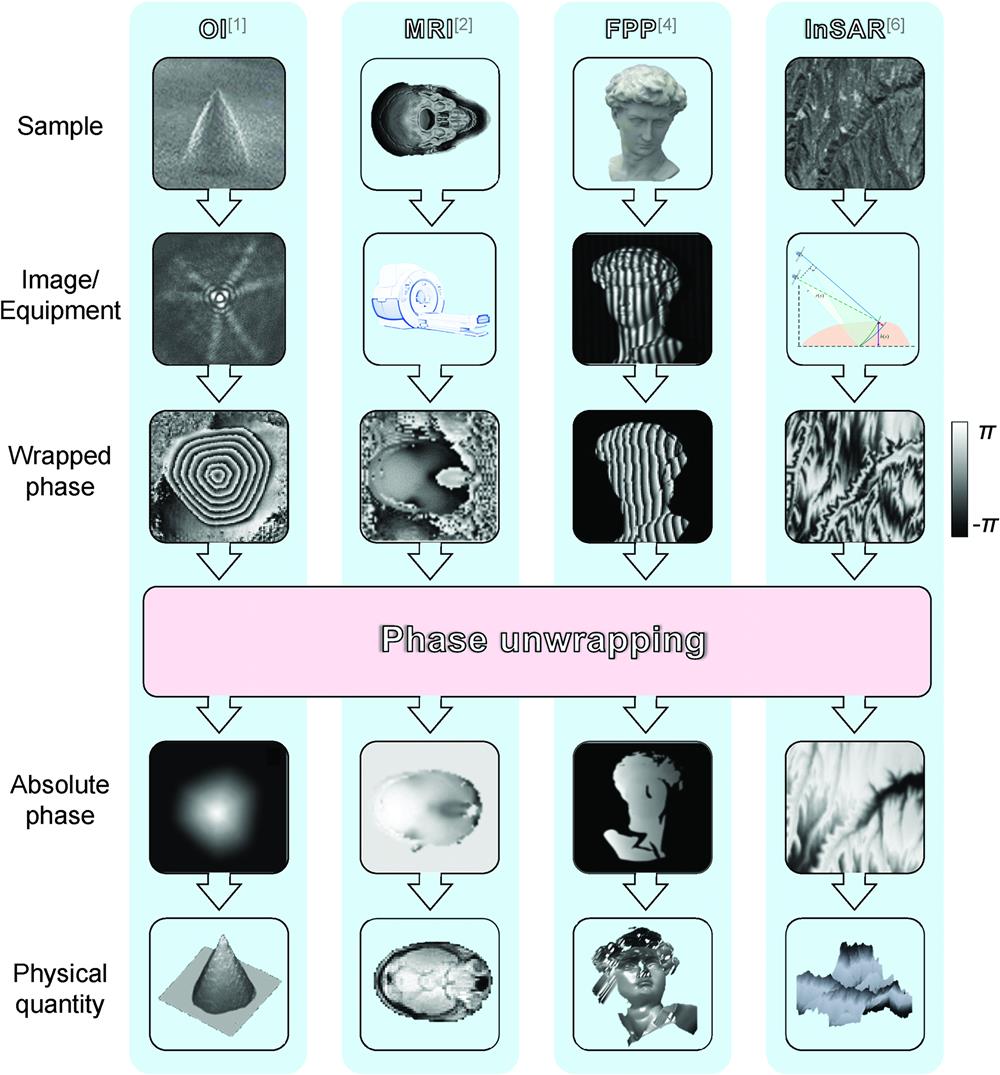
Estimation of absolute (true) phase is an important but challenging problem in many imaging or measurement techniques, such as optical interferometry (OI),1 magnetic resonance imaging (MRI),2 fringe projection profilometry (FPP),3^,4 and interferometric synthetic aperture radar (InSAR)5^,6 (see Fig. 1).

The importance lies in that the estimated absolute phase of the aforementioned applications is directly proportional to the desired physical quantities such as the distribution of thickness or refractive index for OI, the distribution of magnetic susceptibility or the velocity of blood flow for MRI, the three-dimensional (3D) distribution of the object surface for FPP, and the surface height of the topography or ground deformation for InSAR.

The challenge lies in that the initial phase of the aforementioned applications is limited in the range of (−π,π] since it is calculated from the complex amplitude field (CAF) by the arctangent function. However, in most cases, the phase range corresponding to the sample exceeds this limitation. Therefore, to obtain the desired physical quantities, the absolute phase must be estimated from the initial wrapped phase that is the so-called phase unwrapping.

The wrapped phase φ and absolute phase ψ have the following relationship: ψ(r)=φ(r)+2πk(r),(1)where r is the vector coordinate and k is the wrap count, which is an integer.

Spatial phase unwrapping, i.e., getting ψ solely by φ, is straightforward but ill-posed, because both ψ and k are unknown in Eq. (1). However, if the absolute phase is continuous, i.e., the Itoh condition is satisfied, the problem becomes well-posed.7 In the Itoh condition, ψ and φ satisfy the following relationship: ∇ψ=W[∇φ]={∇φ,|∇φ|≤π∇φ−2π,∇φ>π∇φ+2π,∇φ<−π,(2)where W[·] is the wrap operator that removes multiples of 2π so that the output is within [−π,π) and ∇ is the difference operator. Then, the absolute phase can be calculated as ψ(r1)=ψ(r0)+∫L∇ψdr=ψ(r0)+∫LW[∇φ]dr,(3)where r0 is the starting point, r1 is the current point, and L is an arbitrary integration path linking the two points. The simplest integration path is the line-by-line scan.

Unfortunately, in practical applications, noise, discontinuity and aliasing violate the Itoh condition and fail the phase unwrapping. Thus, in the traditional spatial phase unwrapping methods, the path-following method determines better integration paths by branch cuts,8 quality maps,9 etc., to avoid the influence of these invalid pixels, and the optimization-based method obtains the absolute phase by minimizing the difference between absolute phase gradients and wrapped phase gradients, as follows: ψO=argminψt[∬f(∇ψt−W[∇φ])dA],(4)where ψt is the absolute phase field to be optimized, and its optimal value is denoted as ψO; f(·) is an objective function such as energy functions10 and Lp-norm.11 In addition to putting all efforts into improving the unwrapping algorithm, window Fourier transform (WFT) or other filters can be used to filter the noise pixels, with the result denoted as ψF, before phase unwrapping.12^–14 The filtered phase is then unwrapped into ψF. Note that ψO from optimization and ψF with prefiltering are not the same as ψ, thus do not satisfy Eq. (1). Thus, the congruence operation is sometimes applied as14^,15ψC=ψM+W[φ−ψM],(5)where ψM represents any successful but not congruent phase unwrapping results of a particular method, such as ψF and ψO. More details and comparison of the traditional spatial phase unwrapping methods can be found in the classic books and review papers.5^,16^–19

In fact, the purpose of the traditional spatial phase unwrapping methods is to avoid the negative impact of invalid points as much as possible, and it is mainly suitable for nonserious noise and some discrete discontinuous or aliasing points. In some extreme cases such as the presence of severe noise or locally isolated discontinuous or aliasing regions, the traditional methods will become ineffective.

Jin et al.20 first proposed the use of deep learning to solve illposed inverse problems in imaging. This idea of using a deep neural network to learn the mapping relationship from input space to output space from paired datasets makes it possible to solve phase unwrapping in the aforementioned extreme cases. Thus, in the past 4 years, many deep-learning-involved methods have quickly emerged for spatial phase unwrapping that are still effective in the cases of noise, discontinuity, and aliasing due to not being constrained by the Itoh condition.21^–45

These deep-learning-involved methods use different strategies to achieve phase unwrapping by supervised optimization of neural networks with specific datasets:

In addition, the absolute phase dataset generation methods used in deep-learning-involved methods can be divided into the following four categories:

As shown in Fig. 3, the overall process of these deep-learning-involved phase unwrapping methods can be summarized as follows:

Since these methods are proposed individually using different phase unwrapping strategies and dataset generation methods and applied to different scenarios, a comprehensive cross-comparison and a comparison with traditional methods are lacking, which obscures the true potential of deep-learning-involved phase unwrapping and dataset generation methods. In the present review, Sec. 2 offers a summary and classification of deep-learning-involved phase unwrapping methods; in Sec. 3, the dataset generation methods are summarized and classified, their performance and characteristics are compared, and the rules and tips of dataset generation are given; in Sec. 4, using the same dataset, the performance of the deep-learning-involved and traditional phase unwrapping methods in ideal, noisy, discontinuous, aliasing, and mixed cases is compared and summarized; in Sec. 5, the advantages and limitations of the existing deep-learning-involved phase unwrapping methods are summarized, and a deep learning phase unwrapping idea with joint supervision of dataset and physical-model is further proposed and demonstrated.

To give interested readers a quick start, we present a step-by-step guide to applying deep learning to phase unwrapping in the Supplemental Material, with dRG and RME as an example.

Phase unwrapping can be treated as a regression problem in which a neural network directly learns the mapping relationship between the wrapped phase and the absolute phase.22^–33 As illustrated in Fig. 4, after being fed with a wrapped phase, the trained network directly outputs the unwrapped (absolute) phase. Such a mapping relationship is most straightforward and intuitive, but the unwrapped phase does not strictly follow the relationship in Eq. (1). In other words, the unwrapped phase is incongruent, i.e., each pixel has a small error. The congruence operation in Eq. (5) can be applied if necessary.

Dardikman et al.22^,47 introduced the dRG method for simulated steep cells directly through a residual-block-based convolutional neural network (CNN), verified the dRG method with the congruence for real cells and compared the dRG method with the deep-learning-performed wrap count method.23 In 2019, we proposed a phase dataset generation method in which we tested the trained network on real samples, analyzed the network generalization ability by the middle layer visualization, and verified the superiority of the dRG method in noisy and aliasing cases by comparing it with the traditional methods.24^,48 He et al.25 and Ryu et al.26 tested the phase unwrapping performance of the bidirectional recurrent neural network (RNN) and 3D-ResNet with MRI data. Dardikman-Yoffe et al.27 open-sourced their real sample dataset and verified that the congruence could improve the accuracy and robustness of the dRG method in the case of a small number of wrap counts. Qin et al.28 used a larger-capacity Res-UNet to obtain higher accuracy and proposed two evaluation indices. Perera and De Silva29 and Park et al.30 tested the phase unwrapping performance of the long short-term memory (LSTM) network and generative adversarial network (GAN). Zhou et al.31 improved the robustness and efficiency of deep learning phase unwrapping by adding preprocessing and postprocessing. Xu et al.32 improved the accuracy and robustness of phase unwrapping in an end-to-end case by using a composite loss function and adding more skip connections to Res-UNet. Zhou et al.33 used the GAN in InSAR phase unwrapping.

According to Eq. (1), if the wrap counts k(x,y) are successfully determined, the phase unwrapping is also fulfilled by adding 2πk(x,y) to the wrapped phase, as illustrated in Fig. 5. Although the phase values are different from pixel to pixel, the wrap count is the same in one fringe period. Thus, phase unwrapping can be interestingly treated as a classification/segmentation problem in which a neural network predicts the wrap count for each pixel from the wrapped phase.34^–44 Such a mapping relationship is polarized, i.e., it is either correct or incorrect for each pixel.

This idea was introduced by Liang et al.34 and Spoorthi et al.35 Spoorthi et al.35 proposed a phase dataset generation method and used the generated dataset to train a SegNet to predict the wrap count, which was postprocessed by clustering-based smoothness to alleviate the classification imbalance. Zhang et al.36 performed phase unwrapping by three networks sequentially for wrapped phase denoising, wrap count predicting, and postprocessing, respectively. Zhang et al.37^,49 verified the performance of the network DeepLab-V3+ in the dWC method and proposed using refinement for postprocessing. Wu et al.38^,50 enhanced the simulated phase dataset by adding the noise from real data and used the multiscale context and the full resolution residual block (FRRes-UNet) to further optimize the UNet in the Doppler optical coherence tomography. Also, Spoorthi et al. improved the prediction accuracy of the wrap count of the method in Ref. 35 by introducing the priori-knowledge of absolute phase values and gradients into the loss function.39 Zhao et al.40 used a residual autoencoder network (RAEN) to predict the wrap counts, used an image-analysis-based postprocessed method to alleviate the classification imbalance, and adopted iterative-closest-point phase data stitching method to realize dynamic resolution. Zhu et al.41 used the dWC method with postprocessing to do phase unwrapping in inertial confinement fusion target interferometric measurement. Vengala et al.42^,43^,51 used the Y-Net to reconstruct the wrap count and pure wrapped phase at the same time. Zhang and Li44 added atrous spatial pyramid pooling, positional self-attention, and edge-enhanced block to the neural network to get a higher accuracy and stronger robustness.

As mentioned in Sec. 1, in the traditional methods, we can either use complicated algorithms to directly unwrap or circumvent the invalid pixels or filter the invalid pixels before using the simplest algorithm to do phase unwrapping.7^,13^,14 For the latter approach, the neural network can also be used for the invalid pixels filtering.45

Yan et al.45 proposed using a neural network to denoise the real and imaginary parts of CAF for FPP. Then they used the line-scanning method to do phase unwrapping on the noise-filtered wrapped phase. In their work, denoising was performed by extracting the noise components from the noisy real and imaginary parts. After verification, we found that using neural networks to directly extract the pure real and imaginary components had the same performance. Thus, here, we adopt the direct way as shown in Fig. 6. In addition to this way of denoising directly using the neural network, the input of the neural network (the noisy real and imaginary parts) can also be semantically segmented to distinguish the sample area and the background area. Then the semantic segmentation results can be used as prior knowledge to make the neural network focus on the sample area.

For clarity, we summarize all the deep-learning-involved phase unwrapping methods mentioned above in Table 1, where “RME,” “GFS,” “ZPS,” and “RDR” indicate the dataset generation methods, which will be introduced in Sec. 3. In this table, except for the phase unwrapping methods introduced above (column 1), we also include the network structures (column 5), the training datasets (column 6), and the loss functions (column 7), which directly affect the final effect of phase unwrapping.

The network structure is not within the scope of the comparison of this paper, so we choose Res-UNet as a unified network structure that has been widely used in different optical applications with excellent performance.51^–77 Furthermore, the loss functions can be incorporated into the networks as a variable. The dRG and dDN methods usually use mean squared error (MSE) or mean absolute error (MAE) as whole or main components of the loss function, while the dWC method usually uses cross-entropy (CE) as the whole or main component of the loss function. Thus, we use MAE as the loss function of the dRG and dDN, and use CE and MAE as the composite loss function, since which can effectively improve the network accuracy.39

It is well-known that training datasets will affect network performance. Simulation is another convenient and important option for dataset generation, in addition to using real samples to obtain absolute phases. Thus, we will evaluate the effectiveness of the dataset generation methods as a preparation work in Sec. 3, and then compare different phase-unwrapping methods in different cases such as noise, discontinuity, and aliasing in Sec. 4.

In all these comparisons, the following three indices are used for accuracy estimation:

For dRG and dWC, the Res-UNet is selected from Ref. 72 (see Sec. S1 in the Supplemental Material), in which the inception module is introduced into the residual block.24^,47^,51^,78 For dDN, ResNet is obtained by removing the max-pooling and transposed-convolution layers from Res-UNet and changing the channel number of all middle layers to 64. The dWC method is regarded as a classification/segmentation problem of eight categories, including the wrap counts from 0 to 7.

We use the adaptive moment estimation based optimization to train all the networks. The batch size is 16 and the learning rate is 0.01 (85% drop per epoch if the learning rate is >10−6). The epoch size is 100 for all the datasets. The MAE loss function is used for dRG and dDN, while the composite loss function is used for dWC, which can be expressed as Composite loss(r)=1M{−∑m=1MkG(r)log[k(r)]+∑m=1M|ψ(r)−ψG(r)|},(6)where kG(r) is the GT wrap counts, k(r) is the network-output wrap counts, ψG(r) is the GT absolute phases, ψ(r) is the absolute phases obtained from the network-output wrap counts and the network inputs by Eq. (1), and M is the amount of data.

All the networks are implemented by Pytorch 1.0 based on Python 3.6.1, which is performed on a PC with Core i7-8700K CPU, 16 GB of RAM, and NVIDIA GeForce GTX 1080Ti GPU.

Due to the fundamental importance of datasets in deep learning, we introduce the absolute phase generation methods (Sec. 3.1) to prepare the datasets for deep-learning-involved phase unwrapping (Sec. 3.2) and evaluate their richness (Sec. 3.3).

We review three absolute phase generation methods, all of which undergo two steps: generate a random phase and then linearly scale it into a range of [0,h] in radians. For the comparison, here the value range of h is uniformly set from 10 to 40. In practical applications, the range of h can be appropriately enlarged as required. The first step makes these methods different and will be described below, while the second step is the same for all the methods.

The RME method first generates small square matrices with different sizes (randomly set from 2×2 to 8×8), different data distribution types (uniform or Gaussian), and then enlarges them into a size of 128×128 by different interpolation methods (nearest, bilinear, or bicubic interpolation).24^,28^,32 As an example, shown in Fig. 7, an initial small matrix is interpolated and enlarged into a big matrix, which is then linearly mapped to absolute phase with a higher h. In RME, the continuity is guaranteed by interpolation, while the randomness is introduced by the parameter selection of the initial small matrices.

The GFS method generates a random number of Gaussian functions (from 1 to 20) with different means (randomly set from 2 to 127 for x and y directions), variances (randomly set from 100 to 1000) and amplitudes (randomly set from 0 to 1), and then superposes them by addition or subtraction.29^,35^,38^,39^,42^–44 As an example, shown in Fig. 8, three 128×128 Gaussian functions are superposed by addition or subtraction, which are then linearly mapped to absolute phase with a higher h. In GFS, the continuity is guaranteed by using Gaussian functions, while the randomness is introduced by variations of Gaussian parameters and random function superposition.

The ZPS method generates a random number of matrices by the Zernike polynomials with different coefficients (randomly set from 0 to 1) of the first 30 orders (the first coefficient is set to zero), and then superposes these matrices by addition or subtraction.36^,37^,40^,41^,45 The ZPS method is similar to the GFS method except that the Gaussian functions are replaced by Zernike polynomials in which the continuity is guaranteed by Zernike polynomials, while the random strengths of these polynomials introduce the randomness.

The RDR method obtains the absolute phases of real samples and then reprocesses them. The typical ways include: (i) using successful unwrapped results from a traditional phase unwrapping method23^,27^,30^,31^,33; (ii) using optical methods offering absolute phase, such as dual-wavelength (or even multiwavelength) digital holography method79; (iii) using phase-unwrapping-free methods such as the transport of intensity equation (TIE) method.80

Now that the absolute phase ψ has been generated, both the real and imaginary parts of the CAF are calculated as R(x,y)=cos[ψ(r)],(7)I(x,y)=sin[ψ(r)],(8)from which, the wrapped phase φ is calculated as φ(r)=arctan[I(r)/R(r)],(9)and the wrap count is calculated as k(r)=round[ψ(r)−φ(r)2π].(10)We thus obtain the complete dataset as D={ψ,φ,R,I,k}, from which {φ,ψ}, {φ,k}, and {R and I, R and I} are used as the input-GT pairs for dRG, dWC, and dDN, respectively.

Accordingly, we generate the respective datasets denoted as D_RME, D_GFS, and D_ZPS for three different absolute phase generation methods. The simulated datasets in this section do not contain any invalid pixels. As for the real dataset (the fourth dataset, D_RDR), after being obtained by the digital holography and the least squares (LS) phase unwrapping method,11 the absolute phases of real samples are shifted so that the minimum value is equal to zero as the network GT. The wrapped phases are then calculated by Eqs. (7)–(9) as the network input. The real samples contain candle flames, pits of different arrangements, grooves of different shapes, and tables of different shapes. The sizes of the datasets are as follows: for D_RME, D_GFS, and D_ZPS, each contains 20,000 pairs for training and 2000 pairs for testing; D_RDR contains 421 pairs for testing. Given that a higher h corresponds to a more complex wrapped phase, we produce a larger proportion of the data with a higher h. Specifically, for the training part of these three datasets (D_RME, D_GFS, and D_ZPS), the h of 50% data is randomly selected from 10 to 30, 20% from 30 to 35, and 30% from 35 to 40; for the testing part of these three datasets, the h of all data is randomly selected from 10 to 40. The specific information of the datasets can be found in Table 2. Further, we compare the accuracy of the neural networks trained on D_RME and the dataset with a uniform distribution of h (called D_RME0) and find that the former is better (see Sec. S2 in the Supplemental Material).

Shannon entropy,81^,82 as a measurement of the uncertainty of a random variable, can quantitatively characterize the amount of information contained in a dataset, which affects the generalization ability of the trained neural network. We compute the Shannon entropy of the absolute phases from the D_RME, D_GFS, and D_ZPS, as shown in Fig. 9. The means of the entropy from high to low are from RME (mean 4.41), GFS (mean 4.24), and ZPS (mean 4.03). This result gives an initial indication of the better information richness in D_RME and D_GFS.

The gradient (difference) distribution of absolute phases can also reflect the richness of the dataset. Thus, we first calculate the sum of the absolute values of the horizontal difference and vertical difference for each absolute phase in the dataset, and then obtain the statistical average gradient distribution (SAGD) of the dataset. Figure 10 shows the SAGD maps of different datasets, from which we can see that the SAGD values of the four corners of D_RME and D_GSF are low as shown by the red arrow, D_ZPS only has high SAGD value in the four corners as shown in the red circle, and the SAGD value of D_RDR is higher in the lower middle region as shown in the red circle.

We train the same Res-UNet by D_RME, D_GFS, and D_ZPS. As a result, we have three trained networks named RME-Net, GFS-Net, and ZPS-Net, respectively. These three networks are then tested by all the testing datasets and the results are shown in Table 3. We observe that the networks trained with a single type of dataset (RME-Net, GFS-Net, and ZPS-Net) perform best on the test data from the same dataset, and slightly worse on those from other datasets including RDR. This is the so-called generalization problem. For generalization capability, RME-Net is similar to GFS-Net and better than ZPS-Net, which is consistent with the Shannon entropy. What’s more, the congruence operation can significantly improve the accuracy of the networks (see Sec. S3 in the Supplemental Material).

To further analyze the error distribution of the neural network and explore its relationship with the SAGD of the dataset, we calculate the mean error map for each network on each testing dataset. As shown in Fig. 11, RME-Net generalizes well to all testing datasets, GSF-Net generalizes poorly to D_RME, and ZPS-Net generalizes poorly to all non-ZPS testing datasets. This is consistent with the results in Table 3. Furthermore, since the SAGD value on the four corners of D_RME and D_GSF is low but the SAGD value on the four corners of D_ZPS is high, the mean error of RME-Net and GSF-Net on D_ZPS is higher on the four corners as indicated by the small red circles. Similarly, since D_ZPS has a low SAGD value in the regions where the SAGD value of D_RDR is high, the mean error of ZPS-Net on D_RDR is larger in the corresponding regions as indicated by the large red ellipses.

Therefore, the best performing RME method is selected and further improved to obtain a dataset with a uniform SAGD. Specifically, based on the RME method, we enlarge the small square matrices into a size of 160×160 and then intercept the central 128×128 part as the absolute phase, which can avoid a lower SAGD value at the four corners. Using this modified RME method, we generate a dataset of 20,000 pairs of data, called D_RME1, and use it to train the neural network to obtain REM1-Net. As shown in Fig. 12(a), the SAGD map of D_RME1 is more uniform than that of D_RME. Correspondingly, as shown in Fig. 12(b), compared with RME-Net, the mean error of RME1-Net decreases overall, and phase unwrapping can also be performed well for the four corners of the D_ZPS. Likewise, RMSE of RME1-Net is much lower than that of RME-Net (see Sec. S4 in the Supplemental Material).

For more visualization, in Fig. 13, we show the results of RME1-Net for the four testing datasets with the maximum, medians, and minimum RMSEm. Each pixel of the RME1-Net results has a small error, most of which can be corrected by the congruence. The phase unwrapping task is indeed successfully fulfilled by a trained network.

Based on the above evaluation, we select the RME as the dataset generation method to do the following testing for different phase unwrapping methods. Furthermore, the congruence operation is always considered due to its high effectiveness. To facilitate the reader to further understand the deep-learning-involved phase unwrapping, we present a step-by-step example in Sec. S5 of the Supplemental Material, which includes dataset generation, neural network making, training, and testing.

We generate the absolute phase by the RME method. Then Eqs. (7) and (10) are used to get the ideal dataset D={φ,ψ,k}. The pairs {φ,ψ} and {φ,k} are used as input-GT pairs for dRG and dWC, respectively.

To generate the noisy dataset, we add the noise of different degrees to ψ from which other necessary fields are computed. The complete noisy dataset is Dn={ψ,φn,R,I,Rn,In,k}, where the subscript n is used to denote that the fields are noisy, and ψ, R, I, and k remain noiseless. The pairs {φn,ψ}, {φn,k} and {Rn and In, R and I} are used as input-GT pairs for dRG, dWC, and dDN, respectively.

To generate the discontinuity-containing dataset, we place a rectangular area with a random size and phase value of π in ψ from which all other fields are generated in the same way described above. Accordingly, the complete dataset with a discontinuity is Dd={ψd,φd,kd}, where the subscript d is used to denote that the fields are discontinuous. The pairs {φd,ψd} and {φd,kd} are used as input-GT pairs for dRG, and dWC, respectively. dDN is not involved in the comparison.

To generate the aliasing-containing dataset, we simply increase h and the size of the small square matrices to obtain the absolute phase with a steeper distribution. Accordingly, the complete dataset with aliasing is Da={ψa,φa,ka}, where the subscript a is used to denote that the fields are aliasing. The pairs {φa,ψa} and {φa,ka} are used as input-GT pairs for dRG, dWC, respectively. dDN is not involved in the comparison.

To generate the mixed dataset (containing all three of noise, discontinuity, and aliasing), first, we simply increase h and the size of the small square matrices to obtain the absolute phase with a steeper distribution, then place a rectangular area with a random size and phase value of π in ψ, and then add the noise of different degrees to ψ. Accordingly, the mixed dataset is Dm={ψm,φm,km}, where the subscript m is used to denote that the fields are mixed with all three of noise, discontinuity, and aliasing. The pairs {φm,ψm} and {φm,km} are used as input-GT pairs for dRG, dWC, respectively. dDN is not involved in the comparison.

For each noise-containing case, the Gaussian noise with a random standard deviation σn ranging from 0 to 1.8 is added to the pure ψ in which only the data with the wrapped phase SNR≥−3 is kept to eliminate invalid data caused by excessive noise. For each aliasing-free case, when generating datasets, there are 22,000 absolute phases with uniformly distributed h from 10 to 40 in which 20,000 for training and 2000 for testing. For each aliasing-containing case, we set the size of the initial random matrix from 8×8 to 12×12 and set h from 45 to 60. For each discontinuity-containing case, a square area with three random variables is simulated, including the x axis starting point (random value from 1 to 64), the y axis starting point (random value from 1 to 64) and the square size (random value from 20×20 to 50×50); in the square, the phase is set as 2π.

For clarity, Table 4 summarizes the different cases (column 1), the datasets (column 2), the networks (column 3), and the used loss functions (column 4). Due to the increase in h, for each aliasing-free case, the categories number of the network for dWC is increased from 8 to 10, including the wrap counts from 0 to 9. All information about neural network training can be found in Sec. 2.5.

After training, we test the dRG-I and dWC-I. The accuracy evaluation of the networks is shown in Table 5 and Fig. 14. Both dRG with congruence and dWC provide high success rates, with PFS as low as 0.0015 and 0.0025. It should be noted that all three traditional methods, such as line-scanning, congruence of LS, quality guided (QG),10 can get completely correct results, i.e., their PFS is 0. Therefore, on one hand, the deep-learning-involved methods do provide satisfactory results just by some training, and prompt us to further examine and compare them in other more challenging cases; on the other hand, the presence of failed results is annoying, although it is already the state-of-the-art results that we have tried to achieve by now. Ensuring that the neural network can correctly unwrap the wrapped phase with any shape is the focus of future research.

To test the accuracy and adaptation of the neural network to samples with different heights, a testing dataset with h from 1 to 50 is generated by RME to test dRG-I (dRG-I-C) and dWC-I, whose RMSEm is shown in Fig. 15. Note that the networks can successfully complete the phase unwrapping of samples with h<40, but performance degradation occurs for samples with h>40. Further, we train other neural networks by the datasets with h in the range of [10, 80] and perform similar tests, and the height adaptive range of the neural network to h is also increased accordingly (see Sec. S6 in the Supplemental Material), which means that in practical applications, the height range of the training dataset should be appropriately expanded, especially for the upper limit of h.

After training, 2000 pairs of samples in the testing datasets are used to test the corresponding networks, whose accuracy evaluation is shown in Table 6 and Fig. 16. We have the following observations:

To test the performance under different noise levels, we generate another noise-increasing dataset by adding Gaussian noise to five pure absolute phases in which the SNR of the wrapped phase gradually decreases from 20 to −3 in 0.5 intervals. As a comparison, the traditional line-scanning, LS, QG, and window-Fourier-transform-preceded quality guided (WFT-QG) methods are also tested.7^,13^,14 The WFT parameters are selected from a series of values in a range: σx=σy=[3:2:7] for window sizes, ξxl=ξyl=[−0.2:−0.1:−3.0] for low-frequency bounds, ξxh=ξyh=[0.2:0.2:3.0] for high-frequency bounds and thr=[0.2:0.2:6.0] for threshold, where [x:y:z] represents an arithmetic sequence with interval y from x to z; ξxi=1/σx and ξyi=1/σy are accordingly determined for the increasement of frequency.83 This setting produces many parameter combinations, i.e., for each wrapped phase, WFT is applied multiple times with different parameters, and the one with the smallest RMSEm is chosen as the final result. The average RMSEm of these five groups are plotted at different noise levels in Fig. 17. For intuition, we select an example and show the wrapped phase, the absolute phase, the absolute error maps of all the methods in the lower part of Fig. 17. The SNR of each column wrapping phase corresponds to the x axis. We have the following observations:

Deep-learning-involved methods and WFT-QG can cope with the noise level with the wrapped phase SNR as low as 0 or even lower, but WFT-QG needs to be premised on suitable manually found hyperparameters that usually require several attempts. Other traditional methods can only maintain high accuracy in low to medium noise where the SNR of the wrapped phase is >10. It should be noted that dDN-N can also complete the phase unwrapping of ideal samples and obtain an accuracy comparable with dRG-I.

After training, we use the testing datasets to test the corresponding networks and traditional methods, whose accuracy evaluation is shown in Table 7 and Fig. 18. All the indices in Table 7 are calculated from pixels outside the square area. We have the following observations:

After training, we test the dRG-A, dWC-A, line-scanning, LS, and QG methods, whose accuracy evaluation is shown in Table 8 and Fig. 19. We have the following observations:

After training, we test the dRG-M, dWC-M, line-scanning, LS and QG methods, whose accuracy evaluation is shown in Table 9 and Fig. 20. We have the following observations:

Overall, each pixel of the unwrapped phase obtained by dRG and LS has a small error, which can be eliminated by the congruence operation, while the error of the unwrapped phase obtained by dWC, dDN, line-scanning, and QG is either 0 or integer multiples of 2π.

For the ideal case, all traditional methods (line-scanning, LS, and QG) can achieve perfect results, while deep-learning-involved methods (dRG, dWC, and dDN) cannot guarantee perfect completion of phase unwrapping of any shape due to their noninfinite generalization ability. The line-scanning method is most recommended due to its lowest computational cost.

With the introduction of invalid points (noise, discontinuities, and aliasing), the accuracy of deep-learning-involved methods has a corresponding slight drop but is basically lower than that of traditional methods.

For slight noise (SNR>10), all methods can achieve satisfactory results. For moderate and heavy noise (SNR is <10 or even 0), the errors of line-scanning, LS, and QG methods become intolerable, and some errors of the neural network result of dDN will further cause the error propagation of the subsequent line-scanning method. Therefore, dRG, dWC, and WFT-QG are recommended. It should be noted that the unwrapped phase obtained by dWC is noise-containing, while dRG and WFT-QG can first obtain the pure unwrapped phase and, if necessary, the unwrapped phase with noise can be obtained by the congruence operation. The precondition for WFT-QG to obtain the best result is suitable manually found hyperparameters which usually require several attempts.

For discontinuous, aliasing, and even mixed cases, dDN and all traditional methods become powerless due to the Itoh condition, while dRG and dWC can still achieve satisfactory results after targeted training. Therefore, dRG and dWC are recommended as the only options.

To sum up, in Table 10, we present the performance of different methods in the different cases mentioned above.

We have reviewed and compared the phase datasets generation methods (RME, GFS, and ZPS) and deep-learning-involved phase unwrapping methods (dRG, dWC, and dDN). When comparing deep-learning-involved phase unwrapping methods, the traditional methods were also tested for reference. For the dataset selection, the modified RME method is more recommended. The traditional phase unwrapping methods are more reliable and efficient in ideal, slightly, and moderately noisy cases, except WFT-QG, which can get satisfactory accuracy in all noisy cases. The deep-learning-involved methods are more suitable for situations when most of the traditional methods are powerless, such as severe noisy, discontinuous, and aliasing cases.

We aim to provide a relatively uniform and fair condition for different dataset generation methods and phase unwrapping methods. In actual use, the parameter ranges of the three dataset generation methods (such as the initial matrix size in the RME method, the number of Gaussian functions in the GFS method, and the order number of the Zernike coefficient in the ZPS method) can be further expanded for more richness. For the fairness of comparisons and the efficiency of network training, we selected 20,000 as the number of training samples. More samples in practical applications will surely bring further improvement in network performance. In addition to the dataset generation methods mentioned above, the GAN is expected to generate more data based on a small amount of reliable data, thereby further increasing the richness of the dataset.84 Once the training is complete, the size of the neural network input is fixed to the size of the training data. In practical applications, the size of the data to be unwrapped is generally different from that of the neural network input. To dynamically adapt the resolution, we propose to first divide the entire data into multiple overlapping subregions of fixed size, then do phase unwrapping for each subregion by the neural network, and finally use the stitching algorithm to obtain the entire absolute phase.40^,85^,86

The neural networks used in the above comparations are all based on Res-UNet. Some other types of network structures (such as Bayesian network,87 dynamic convolution,88 and attention UNet89) may further improve the accuracy of phase unwrapping.

All the deep-learning-involved methods mentioned in this paper rely on dataset supervision to learn the mapping relationship from input to GT. The wrapped phase can be unwrapped by passing through the trained neural network only once, but its generalization ability for samples with different shapes is not infinite.

Different types of objects contain different shape features in their phase distributions. For example, as a common object of interferometry, the phase distribution of the lens surface has a style of slow fluctuation and low-frequency information. As a common object of InSAR, the phase distribution of mountainous terrain has a style of obvious tortuous and high-frequency information. As a common object of holographic microscopy, the phase distribution of cells usually has a style that considers both high-frequency and low-frequency information. Therefore, we believe that a promising way to solve the problem of generalization ability is transfer learning.90 The transfer learning way is, first, pretraining a standard neural network with a simulated dataset; then, for a specific target object, using the real dataset of this type of object to fine-tune the neural network; finally, unwrapping the wrapped phase through the fine-tuned neural network at one time.

But what if there is no real dataset of the target object? Different from the dataset-supervision method, inspired by deep image priori,91 Yang et al.92 used the Itoh condition to guide the convergence of the neural network as a physical-model supervision method, without GT and with stronger generalization ability for samples with different shapes. However, the initialized network does not include any mapping relationship from the wrapped phase to the absolute phase, leading to a large number of iterations for each phase unwrapping. Similar to transfer learning, we propose to combine the dataset supervision with physical-model supervision, which can significantly reduce the number of iterations. That is, pretraining the neural network by the simulation-generated dataset, and then fewer iterations are required for the physical-model supervision method.

Here, we show the preliminary results of this idea. To make the input and the neural network related, we change the input of the neural network in Ref. 92 from a random vector to a wrapped phase. We use the method in Sec. 4.1 to generate a training dataset containing 50,000 pairs of data, D={φ,ψ}, and then randomly take out 5000, 500, and 50 pairs as the other three training datasets.

As shown in Fig. 21, by the pretrain loss function, Pretrain loss=‖∇[f(φ)]−∇[ψ]‖,(11)we use the four training datasets to pretrain Res-UNet. Then, the four pretrained Res-UNets are used to unwrap a wrapped phase by the physical-model supervision with the following retrain loss function: Retrain loss=‖W[∇φ]−∇[f(φ)]‖.(12)For comparison, we also use the physical-model supervision to train an initialized Res-UNet without pretraining.

From the retrain loss plot of the five networks shown in Fig. 22, we can find that the convergence speed of the pretrained networks is significantly faster than the initialized one without pretraining. Specifically, the initialized network without pretraining requires 500 epochs to converge, while the pretrained neural networks can converge in <100 epochs with higher precision. It is more interesting that with only one pretraining by the dataset of 50 pairs, the epoch required to achieve the same accuracy can be reduced from 500 to 32; further, by increasing the pretraining datasets of 50 pairs to 50,000 pairs, the required epoch also reduces from 32 to 17.

This idea of pretraining with dataset supervision and then retraining with physical-model supervision also has great potential in other fields, such as phase imaging,93 coherent diffractive imaging,94 and holographic reconstruction.95

Kaiqiang Wang received the bachelor’s and PhD degrees from the Northwestern Polytechnical University in 2016 and 2022, respectively. His research interests include computational imaging and deep learning.

Qian Kemao is currently an associate professor at the School of Computer Science and Engineering, Nanyang Technological University, Singapore. He received his bachelor’s, master’s, and PhD degrees from the University of Science and Technology of China in 1994, 1997, and 2000, respectively. He has published more than 150 scientific articles and a monograph. His research interests include optical metrology, image processing, computer vision, and computer animation.

Jianglei Di is currently a professor at the School of Information Engineering, Guangdong University of Technology, Guangzhou, China. He received his BS, MS, and PhD degrees from NPU in 2004, 2007, and 2012, respectively. His research interests include digital holography, optical information processing, optical precision measurement and deep learning.

Jianlin Zhao is currently a professor at the School of Physical Science and Technology, Northwestern Polytechnical University (NPU), Xi’an, China. He received his BS and MS degrees from NPU in 1981 and 1987, respectively. He received his PhD in optics from Xi’an Institute of Optics and Precision Mechanics, Chinese Academy of Sciences, Xi’an, in 1998. He is the director of Shaanxi Key Laboratory of Optical Information Technology, and MOE Key Laboratory of Material Physics and Chemistry under Extraordinary Conditions. His research interests include light field manipulation, imaging, information processing, and applications.