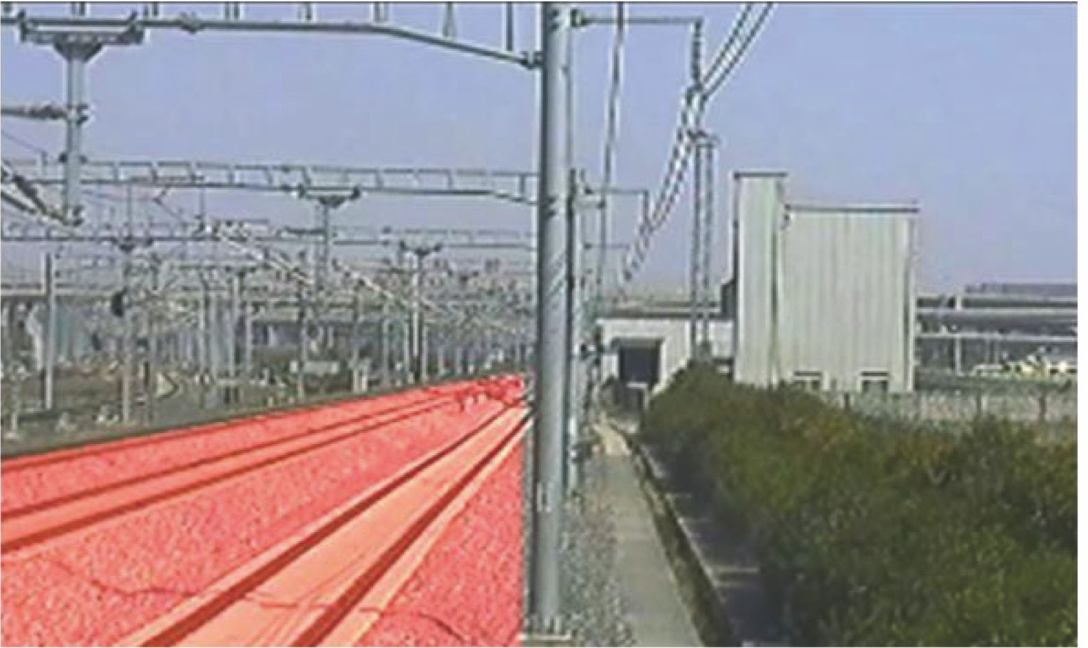
Fig. 1. Railway scene and track area

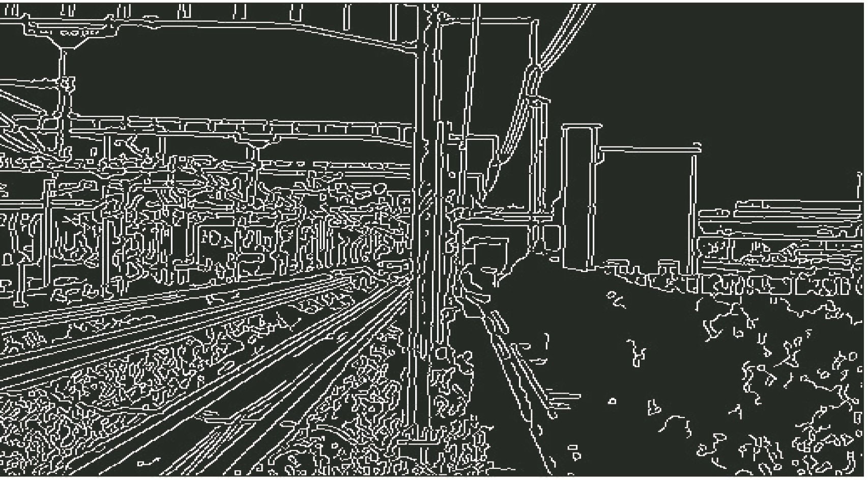
Fig. 2. Edge feature map of railway scene

Fig. 3. Distribution of linear character after Hough transformation

Fig. 4. Gaussian convolution kernels rotated by adaptive angles. (a) θ=22°; (b) θ=38°; (c) θ=90°; (d) θ=178°

Fig. 5. Procedures of combining fragmented regions. (a) Strong and weak boundaries; (b) distribution of boundary weight; (c) boundaries after deletion of weak points; (d) fragmented regions; (e) distribution of fragmented region area; (f) local areas after combination; (g)-(o) local areas after segmentation

Fig. 6. Schematic of convolutional neural network structure

Fig. 7. Pre-train convolutional kernels using autoencoder network. (a) Structure of autoencoder networks; (b) pre-trained convolution kernels

Fig. 8. Structural schematic of high-speed railway intrusion detecting system

Fig. 9. Comparison diagrams of results of different algorithms for track area recognition. (a) Railway scenes; (b) manually labeled regions; (c) results of MCG algorithm; (d) results of FCN algorithm; (e) results of proposed algorithm

Table 1. Comparison of experimental results of different CNN network structures

Table 2. Comparison of experimental results of different convolutional neural network structures after optimization

Table 3. Comparison of experimental results of different algorithms