Researching | Uniform-velocity spacetime crystals

Journals >Advanced Photonics >Volume 1 >Issue 5 >Page 056002 > Article

Advanced Photonics
Vol. 1, Issue 5, 056002 (2019)

Uniform-velocity spacetime crystals

Zoé-Lise Deck-Léger^1、*, Nima Chamanara¹, Maksim Skorobogatiy², Mário G. Silveirinha³, and Christophe Caloz¹

Author Affiliations

¹Polytechnique Montréal, Department of Electrical Engineering, Montréal, Quebec, Canada

²Polytechnique Montréal, Department of Engineering Physics, Montréal, Quebec, Canada

³Universidade de Lisboa - Instituto Superior Técnico and Instituto de Telecomunicações, Department of Electrical Engineering, Lisbon, Portugal

show less

DOI: 10.1117/1.AP.1.5.056002 Cite this Article Set citation alerts

Zoé-Lise Deck-Léger, Nima Chamanara, Maksim Skorobogatiy, Mário G. Silveirinha, Christophe Caloz. Uniform-velocity spacetime crystals[J]. Advanced Photonics, 2019, 1(5): 056002 Copy Citation Text

show less

$Representation of two canonical spacetime crystals. Here, the variable z is intended to represent the hyperspace, i.e., the three dimensions of space. The white and gray regions correspond to media with refractive indices ni and nj, respectively. (a) Double-period (pA and pB) structure, characterized by two velocities, υm1 and υm2, which may be interpreted as acceleration at the corner. (b) Single-period (p) structure, characterized by a unique and uniform velocity, υm.$

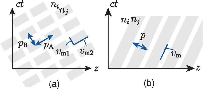
Fig. 1. Representation of two canonical spacetime crystals. Here, the variable

z

is intended to represent the hyperspace, i.e., the three dimensions of space. The white and gray regions correspond to media with refractive indices

n_{i}

and

n_{j}

, respectively. (a) Double-period (

p_{A}

and

p_{B}

) structure, characterized by two velocities,

υ_{m 1}

and

υ_{m 2}

, which may be interpreted as acceleration at the corner. (b) Single-period (

p

) structure, characterized by a unique and uniform velocity,

υ_{m}

.

Download full size | View in the Article

$Scattering at a spacetime interface. The white and gray regions correspond to media i and j, with refractive indices ni and nj (ni<nj). (a) Sketch of a wave incident on a subluminal interface. (b) Same as (a) but for a superluminal interface. (c) Scattering from a subluminal (υm<c) interface in a spacetime diagram. The blue arrows represent wave trajectories (referring to a specific phase point of the waveform), and the black arrows represent scattering coefficients. The dashed lines correspond to incidence from the right. The laboratory and moving frames are superimposed with common origin, and the moving frame has the same velocity as the interface (υf/c=υm/c). (d) Same as (c) but for a superluminal interface (υm>c), with moving frame having the inverse velocity of the interface (υf/c=c/υm).$

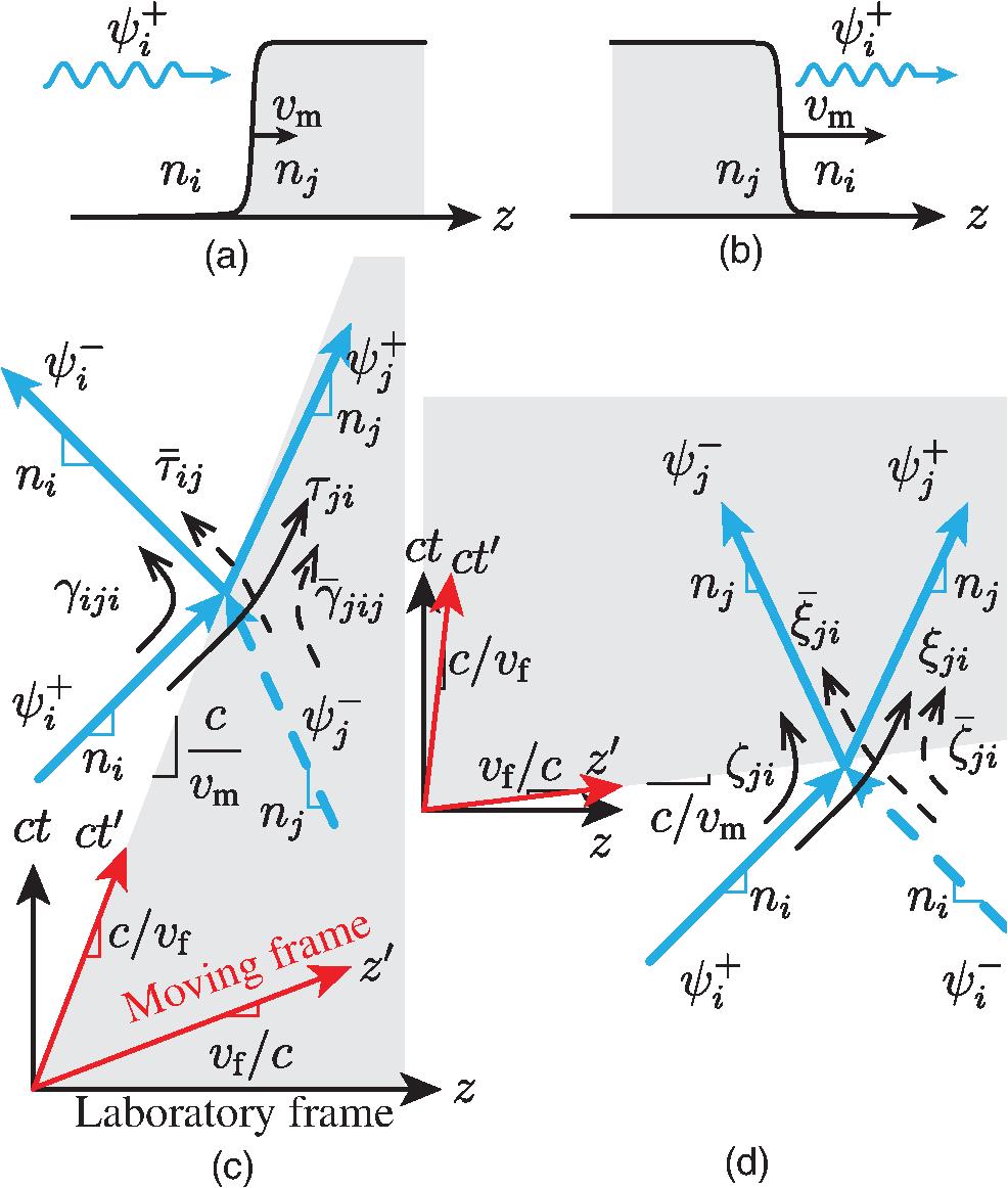
Fig. 2. Scattering at a spacetime interface. The white and gray regions correspond to media

i

and

j

, with refractive indices

n_{i}

and

n_{j}

(

n_{i} < n_{j}

). (a) Sketch of a wave incident on a subluminal interface. (b) Same as (a) but for a superluminal interface. (c) Scattering from a subluminal (

υ_{m} < c

) interface in a spacetime diagram. The blue arrows represent wave trajectories (referring to a specific phase point of the waveform), and the black arrows represent scattering coefficients. The dashed lines correspond to incidence from the right. The laboratory and moving frames are superimposed with common origin, and the moving frame has the same velocity as the interface (

υ_{f} / c = υ_{m} / c

). (d) Same as (c) but for a superluminal interface (

υ_{m} > c

), with moving frame having the inverse velocity of the interface (

υ_{f} / c = c / υ_{m}

).

Download full size | View in the Article

Fig. 3. Spacetime-inversion symmetry of subluminal (SUB) and superluminal (SUP) structures. (a) Interfaces. (b) Slabs.

Download full size | View in the Article

Fig. 4. Graphical description of the interluminal regime in spacetime diagram. (a) Codirectional case, with a single scattered wave. (b) Contradirectional case, with three scattered waves.

Download full size | View in the Article

Fig. 5. Generalization of the Stokes principle. (a) Subluminal regime. (b) Superluminal regime.

Download full size | View in the Article

Fig. 6. Frequency transitions at a spacetime interface corresponding to Fig. 2. (a) Subluminal case. (b) Superluminal case.

Download full size | View in the Article

Fig. 7. Multiple-reflection description of the scattering phenomenology in spacetime slabs. Changes in line type (solid

\leftrightarrow

dashed) denote phase reversals. (a) Subluminal slab, with phase change occurring upon reflection to a lower impedance medium (

η_{j} < η_{i}

), according to Eqs. (18). Note that the slope of the trajectories has been altered for representation convenience. (b) Superluminal slab, with phase change occurring upon reflection to a higher impedance medium (

η_{k} > η_{j}

), according to Eqs. (22).

Download full size | View in the Article

Fig. 8. Graphical Bragg-like interference argument. The light and dark blue trajectories correspond to the maxima and minima of the incident wave, and changes in line type (solid

\leftrightarrow

dashed) denote phase reversals. (a) Subluminal case, with constructive and destructive interference in reflection and transmission, respectively. Note that the slope of the trajectories has been altered for representation convenience. (b) Superluminal case, with constructive interference in both the later forward and later backward waves.

Download full size | View in the Article

Fig. 9. Bilayer spacetime crystal with spacetime unit cell and out-of-gap wave trajectories. (a) Subluminal equal-length crystal, with

ℓ_{1} = ℓ_{2}

. The slopes of the triangles ① and ② are

n_{1} = c t_{1}^{+} / z_{1}^{+}

and

n_{2} = c t_{2}^{+} / z_{2}^{+}

, so

z_{1}^{+} = c t_{1}^{+} / n_{1}

and

z_{2} = c t_{2}^{+} / n_{2}

. Substituting these lengths into the expression for the slope

n_{av} = (c t_{1}^{+} + c t_{2}^{+}) / (z_{1}^{+} + z_{2}^{+})

, yields Eq. (51). (b) Superluminal equal-duration crystal, with

d_{1} = d_{2}

. From the slopes of the triangles ① and ②, given in (a), we have

c t_{1}^{+} = z_{1}^{+} n_{1}

and

c t_{2} = z_{2}^{+} n_{2}

. Substituting these durations into the expression for the average slope, also given in (a), yields Eq. (55).

Download full size | View in the Article

Fig. 10. Linear approximation of the dispersion diagram of bilayer crystals with

n_{2} / n_{1} = 1.5

and equal electrical lengths. (a) Subluminal case, with

υ = (1 / 3) c

. (b) Superluminal case, with

υ = 2 c

.

Download full size | View in the Article

Fig. 11. Bilayer spacetime crystal with spacetime unit cell. (a) Subluminal regime. (b) Superluminal regime.

Download full size | View in the Article

Fig. 12. Dispersion diagram of bilayer crystals with

n_{2} / n_{1} = 1.5

and equal phases (

{\bar{φ}}_{j} = {\bar{φ}}_{k}

). The solid curves correspond to the exact solution [Eqs. (86) and (89)], with the black and blue parts, respectively, corresponding to the real and imaginary parts, and the dashed curves to the linear approximation [Eq. (63)]. (a) Subluminal case, with

υ = (1 / 3) c

. (b) Superluminal case, with

υ = 3 c

.

Download full size | View in the Article

Fig. 13. Examples of spacetime crystal truncation by a pair of spactime interfaces of velocities

υ_{L}

and

υ_{R}

for the left and right interfaces, respectively. Top row: the two interfaces have the same velocity,

υ_{L} = υ_{R}

. Bottom row: the two interfaces have different velocities,

υ_{L} \neq υ_{R}

. (a) Purely spatial truncation,

υ_{L} = υ_{R} = 0

. (b) Truncation with velocity different from the modulation velocity,

υ_{L} = υ_{R} \neq υ_{m}

. (c) Comoving truncation,

υ_{L} = υ_{R} = υ_{m}

. (d) Antiparallel truncation,

υ_{L} \neq υ_{R} \neq υ_{m}

. (e) Spacetime cavity with piecewise constant velocities. (f) Spacetime cavity with continuously varying velocity.

Download full size | View in the Article

$Scattering from two canonical truncated spacetime crystals. In both cases, the crystal is subluminal, and the medium surrounding it is a simple nondispersive dielectric medium of refractive index n0. Top row: dispersion diagrams with transition frequencies. Bottom row: spacetime diagrams with scattered waves, with labels corresponding the solutions of the top panels. Note that the drawn scattered waves correspond to the waves seen in the laboratory frame and would completely different in the moving frame. (a) Comoving truncation. A moving-frame observer would see a stationary crystal bounded by stationary interfaces, and hence measure a unique frequency everywhere, inside and outside the crystal. The arrows indicate the up and down frequency and wavenumber transitions at the two interfaces. (b) Purely spatial truncation. A moving-frame observer would see a stationary crystal bounded by moving interfaces, and hence measure an infinity of frequencies.$

Fig. 14. Scattering from two canonical truncated spacetime crystals. In both cases, the crystal is subluminal, and the medium surrounding it is a simple nondispersive dielectric medium of refractive index

n_{0}

. Top row: dispersion diagrams with transition frequencies. Bottom row: spacetime diagrams with scattered waves, with labels corresponding the solutions of the top panels. Note that the drawn scattered waves correspond to the waves seen in the laboratory frame and would completely different in the moving frame. (a) Comoving truncation. A moving-frame observer would see a stationary crystal bounded by stationary interfaces, and hence measure a unique frequency everywhere, inside and outside the crystal. The arrows indicate the up and down frequency and wavenumber transitions at the two interfaces. (b) Purely spatial truncation. A moving-frame observer would see a stationary crystal bounded by moving interfaces, and hence measure an infinity of frequencies.

Download full size | View in the Article

Fig. 15. Transmission and reflection coefficients for an

N = 15

-layer crystal [corresponding to Fig. 13(c) and Fig. 14(a)] with

{\bar{ϕ}}_{1,2} = π / 2

. The gap centers

ω_{i}

,

k_{i}

are provided in Appendix E (Sec. 12). (a) Subluminal case, with

υ = 1 / 3 c

and

n_{2} / n_{1} = 2

, with attenuation in the bandgaps. (b) Superluminal case, with

υ = 3 c

and

n_{2} / n_{1} = 1.2

with amplification in the bandgaps.

Download full size | View in the Article

Fig. 16. Spacetime interface represented in two inertial frames. The arrows represent the trajectories of the media particles. In both (a) and (b), the interfaces of the spacetime variation are parallel to the

c t^{'}

axis and the media trajectories are parallel to the

c t

axis. (a) Laboratory frame viewpoint. Media appear at rest. Wave velocity is independent of direction:

υ_{j}^{+} = υ_{j}^{-}

(b) Moving frame viewpoint. Media appear to be moving in

- z

direction. Wave velocities are direction dependent:

υ_{j}^{+} \neq υ_{j}^{-}

, with

| υ_{j}^{-} | > | υ_{j}^{+} |

.

Download full size | View in the Article

Fig. 17. Graphical derivation of the travel length or duration across the unit cell of the crystal. (a) Subluminal regime (length). (b) Superluminal regime (duration).

Download full size | View in the Article

Fig. 18. Successive application of time reversal (

T

) and space reversal (

P

).

Download full size | View in the Article

Fig. 19. Construction to find the frequencies aligned with the bandgaps. (a) Subluminal regime. (b) Superluminal regime.

Download full size | View in the Article


Subluminal regime	Superluminal regime
Space	$z$	Time	$c t$
Time	$c t$	Space	$z$
Modulation velocity	$v_{m} / c$	Inverse velocity	$c / v_{m}$
Refractive index	$n$	Inverse index	$1 / n$
Phase velocity	$v / c = 1 / n$	Inverse phase velocity	$c / v = n$
Length	$ℓ$	Duration	$c d$
Wavelength	$λ$	Period	$c T$
Frequency	$ω / c$	Wavenumber	$k$

Table 1. Duality transformations between the subluminal and superluminal regimes.

View in the Article


Subluminal	Superluminal
Coefficients (Fig. 2)
$τ_{j i} = \frac{2 η_{j}}{η_{i} + η_{j}} (\frac{1 - α_{i}}{1 - α_{j}})$ [Eq. (18b)]	$ξ_{j i} = \frac{η_{i} + η_{j}}{2 η_{i}} (\frac{1 - α_{i}}{1 - α_{j}})$ [Eq. (22b)]
$γ_{i j i} = \frac{η_{j} - η_{i}}{η_{i} + η_{j}} (\frac{1 - α_{i}}{1 + α_{i}})$ [Eq. (18a)]	$ζ_{j i} = \frac{η_{i} - η_{j}}{2 η_{i}} (\frac{1 - α_{i}}{1 + α_{j}})$ [Eq. (22a)]
Frequencies (Fig. 6)
$ω_{i}^{-} = ω_{i}^{+} \frac{1 - α_{i}}{1 + α_{i}}$ [Eq. (26b)]	$k_{j}^{-} = k_{i}^{+} \frac{1 - 1 / α_{j}}{1 + 1 / α_{i}}$ [Eq. (28b)]
$ω_{j}^{+} = ω_{i}^{+} \frac{1 - α_{i}}{1 - α_{j}}$ [Eq. (26b)]	$k_{j}^{+} = k_{i}^{+} \frac{1 - 1 / α_{i}}{1 - 1 / α_{i}}$ [Eq. (28b)]
$α_{i, j} = v_{m} / v_{i, j}$

Table 2. Summary of the scattering formulas, derived in Sec. 3, for a spacetime interface.

View in the Article


Subluminal regime	Superluminal regime
Phase (Fig. 7)
$φ_{j}^{\pm'} = {\bar{φ}}_{j}^{'} \pm Δ φ_{j}^{'}$ [Eq. (35a)]
${\bar{φ}}_{j} = ω_{e} ℓ_{j} \frac{v_{j}}{v_{j}^{2} - v_{m}^{2}}$ [Eq. (38b)]	${\bar{φ}}_{j} = k_{e} d_{j} \frac{v_{j} v_{m}^{2}}{v_{j}^{2} - v_{m}^{2}}$ [Eq. (41b)]
$Δ φ_{j} = \frac{{\bar{φ}}_{j} γ^{2} (1 - v_{j}^{2} / c^{2}) v_{m}}{v_{j}}$ [Eq. (38c)]	$Δ φ_{j} = \frac{{\bar{φ}}_{j} γ^{2} (1 - v_{j}^{2} / c^{2}) c^{2}}{v_{j} v_{m}}$ [Eq. (41c)]
Coefficients (Fig. 7)
$Γ_{i k i} = γ_{i j i} \frac{1 - e^{2 i {\bar{φ}}_{j}}}{1 - {\bar{γ}}_{j i j} γ_{j k j} e^{2 i {\bar{φ}}_{j}}}$ [Eq. (42)]	$Z_{k i} = ζ_{k j} ξ_{j i} e^{- i φ_{j}^{-}} (e^{i {\bar{φ}}_{j}} - 1)$ [Eq. (47)]
$T_{k i} = \frac{τ_{k j} τ_{j i} e^{i φ_{j}^{+}}}{1 - {\bar{γ}}_{j i j} γ_{j k j} e^{2 i {\bar{φ}}_{j}}}$ [Eq. (44)]	$Ξ_{k i} = [1 + ξ_{k j} ξ_{j i} (e^{i {\bar{φ}}_{j}} - 1)] e^{- i φ_{j}^{-}}$ [Eq. (47)]
Bragg interference condition (Fig. 8)
$ℓ_{j} = \frac{λ_{j}^{+}}{4} (1 + \frac{v_{m}}{v_{j}})$ [Eq. (49)]	$d_{j} = \frac{T_{j}^{+}}{4} (1 + \frac{v_{j}}{v_{m}})$ [Eq. (50)]

Table 3. Summary of spacetime slab results.

View in the Article


Modulation regime	Velocity ( $v_{m}$ )	Average index ( $n_{av}^{+}$ )	Average index ( $n_{av}^{-}$ )
Spatial	0	$\frac{1}{2} (n_{1} + n_{2})$	$\frac{1}{2} (n_{1} + n_{2})$
Subluminal upper limit	$v_{2} = \frac{c}{n_{2}}$	$n_{2}$	$n_{2} \frac{3 n_{1} + n_{2}}{n_{1} + 3 n_{2}}$
Superluminal lower limit	$v_{1} = \frac{c}{n_{1}}$	$n_{1}$	$n_{1} \frac{3 n_{2} + n_{1}}{n_{2} + 3 n_{1}}$
Temporal	$\infty$	$\frac{1}{2} {(\frac{1}{n_{1}} + \frac{1}{n_{2}})}^{- 1}$	$\frac{1}{2} {(\frac{1}{n_{1}} + \frac{1}{n_{2}})}^{- 1}$

Table 4. Average refractive index for different modulation velocities, from (53), with

ℓ_{1} = ℓ_{2}

(upper half) and Eq. (57), with

d_{1} = d_{2}

(lower half).

View in the Article

Figures&Tables (23)

Equations (169)

References (68)

Copy Citation Text

Zoé-Lise Deck-Léger, Nima Chamanara, Maksim Skorobogatiy, Mário G. Silveirinha, Christophe Caloz. Uniform-velocity spacetime crystals[J]. Advanced Photonics, 2019, 1(5): 056002

Download Citation

Set citation alerts for the article

Set citation alerts for the article

Save the article for my favorites

Paper Information

Recommended Topics

laser devices and laser physics

Lasers and Laser Optics

laser manufacturing

Instrumentation, Measurement and Metrology

Set citation alerts for the article

Please enter your email address