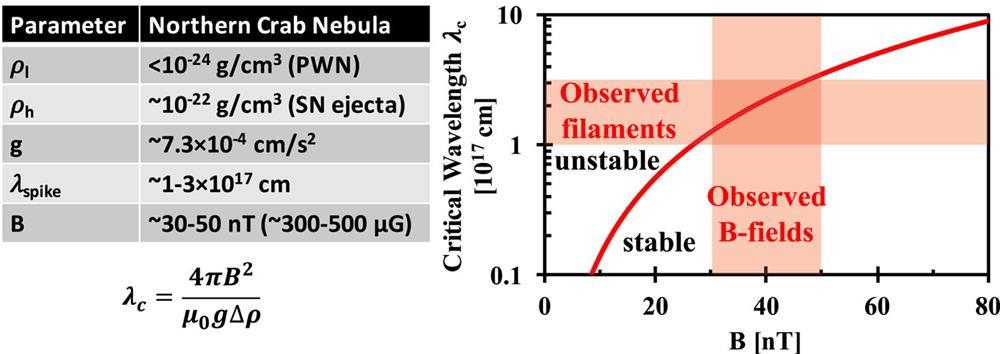
Fig. 1. Critical wavelength plotted as a function of B-field strength for Rayleigh–Taylor (RT)-relevant parameters in the northern edge of the Crab Nebula. In this system, the low-density pulsar wind nebula (PWN) pushes on the high-density supernova (SN) ejecta.

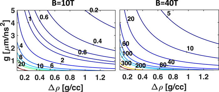
Fig. 2. Contour plots of λ_c (μm) as a function of Δρ and g for typical parameter ranges found in laser-driven experiments with a 10-T or 40-T B-field aligned parallel to the wave vector in the ideal-MHD limit.

Fig. 3. (a) Schematic of physics package, laser drive, and B-field orientation across rippled interface. (b) Experimental setup showing x-ray radiography configuration with B-field now out of the page. Streaked self-emission is also collected with a field of view aligned with the shock tube to measure interface velocity. (c) Predicted density distributions from resistive- and ideal-MHD simulations at 20 ns illustrating the effect of a 10-T B-field on the RT evolution in LULI experiments under varying resistivities. (d) Shock position (similar in all cases) and peak-to-valley (P–V) amplitudes plotted as a function of time. The cases of B = 0 T and nominal Spitzer resistivity overlap, as suggested by the images shown in (c). Under ideal-MHD conditions, the P–V amplitude deviates significantly from that in the unmagnetized and nominal-Spitzer cases.

Fig. 4. (a) Radiographs from flat CHI experiments at three different times with and without the 10-T B-field. (b) Experimental positions of the CHI interface from radiographs for B = 0 T (blue squares) and B = 10 T (red circles). Ideal-MHD FLASH calculations (solid lines) predict no difference in the interface position and fit parabolic trajectories (dotted lines past 30 ns). The high-opacity (dark gray) region near the bottom of each x-ray radiograph is caused by mid-Z shielding near the base of the target.

Fig. 5. Streaked optical emission data for a B = 0 T shot with the simulated CHI trajectory (solid line) and extrapolated parabolic fit (dotted line). Expansion of the CHI begins to cause deviation from the parabolic fit for t ≳ 30 ns. Consistent with the radiographic data from flat CHI experiments, the typical streaked emission data are unchanged upon adding a 10-T B-field.

Fig. 6. (a) Experimental x-ray radiographs of CHI foils with machined sinusoidal perturbations with wavelength λ = 120 μm and initial P–V amplitude 20 μm. (b) Measurements of P–V amplitude as a function of time for experiments with (red circles) and without (blue circles) a 10-T B-field. FLASH simulation results from Fig. 3 are shown as well.

Fig. 7. B-field distributions (T) from ideal- and resistive-MHD FLASH calculations. Ideal MHD predicts >10× increase in B-field strength, whereas a Spitzer model in resistive MHD shows an increase of ∼ 2×.

Fig. 8. Scanning electron microscope images of different versions of GACH: (a) 8.5-mg/cc GACH foam used in this work, showing sub-micron pore structure; (b) 30-mg/cc GACH showing uniform distribution of ZnO nanoparticles; (c) shard from a GACH sphere coated with 5 μm of solid gas-discharge-polymer (GDP), showing no penetration of the coating material into the foam structure.

Fig. 9. (a) X-ray radiograph of undriven target showing foam-filled shock tube; the CHI is obscured by the shielding. (b) Lineouts of mesh in near-axial and near-radial directions show an isotropic magnification of 17.2. (c) A Gaussian blur with a standard deviation of 11 pixels fits the knife-edge data and corresponds to a 2σ resolution of ∼32 μm.

Table 1. Nominal parameters for northern rim of Crab Nebula^5–7,15,36 and LULI experiments.