
Ming Chen, Xiangyun Xi, Yang Wang. Hyperspectral Image Classification Based on Residual Generative Adversarial Network[J]. Laser & Optoelectronics Progress, 2022, 59(22): 2210008
- Laser & Optoelectronics Progress
- Vol. 59, Issue 22, 2210008 (2022)
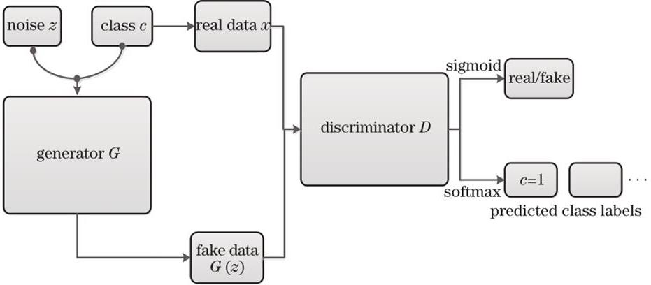
Fig. 1. Framework of GAN for hyperspectral image classification
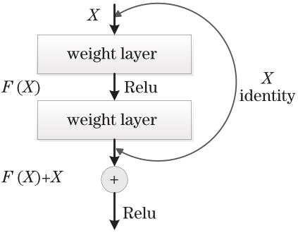
Fig. 2. Sructure of residual unit
Fig. 3. Flowchart of hyperspectral image classification method using residual generative adversarial network
Fig. 4. Structure for residual block of generator
Fig. 5. Network structure of generator
Fig. 6. Structure for residual block of discriminator. (a) Block structure with convolution residuals; (b) Block structure without convolution residuals
Fig. 7. Network structure of discriminator
Fig. 8. Pavia University dataset. (a) Pseudo color image; (b) ground datum map
Fig. 9. Salinas dataset. (a) Pseudo color image; (b) ground datum map
Fig. 10. Indian Pines dataset. (a) Pseudo color image; (b) ground datum map
Fig. 11. Hyperspectral image classification result map of Indian Pines dataset. (a) CAE-SVM; (b) 2DCNN; (c) 3DCNN; (d) ResNet;(e) proposed method
Fig. 12. Hyperspectral image classification result map of Pavia University dataset. (a) CAE-SVM; (b) 2DCNN; (c) 3DCNN; (d) ResNet;(e) proposed method
Fig. 13. Hyperspectral image classification result map of Salinas dataset. (a) CAE-SVM; (b) 2DCNN; (c) 3DCNN; (d) ResNet;(e) proposed method
|
Table 1. Categories and number of Pavia University hyperspectral dataset
|
Table 2. Categories and number of Salinas hyperspectral dataset
|
Table 3. Categories and number of Indian Pines dataset
| |||||||||||||||||||||||||||||||||||||||||||||||||||||||||||||||||||||
Table 4. Comparison of classification results of ablation experiments
|
Table 5. Comparison of classification accuracy of Indian Pines hyperspectral dataset
|
Table 6. Comparison of classification accuracy of Pavia University hyperspectral dataset
|
Table 7. Comparison of classification accuracy of Salinas hyperspectral dataset

Set citation alerts for the article
Please enter your email address
© Copyright 2018-2021 | Chinese Laser Press. All Rights Reserved 沪ICP备15018463号-20