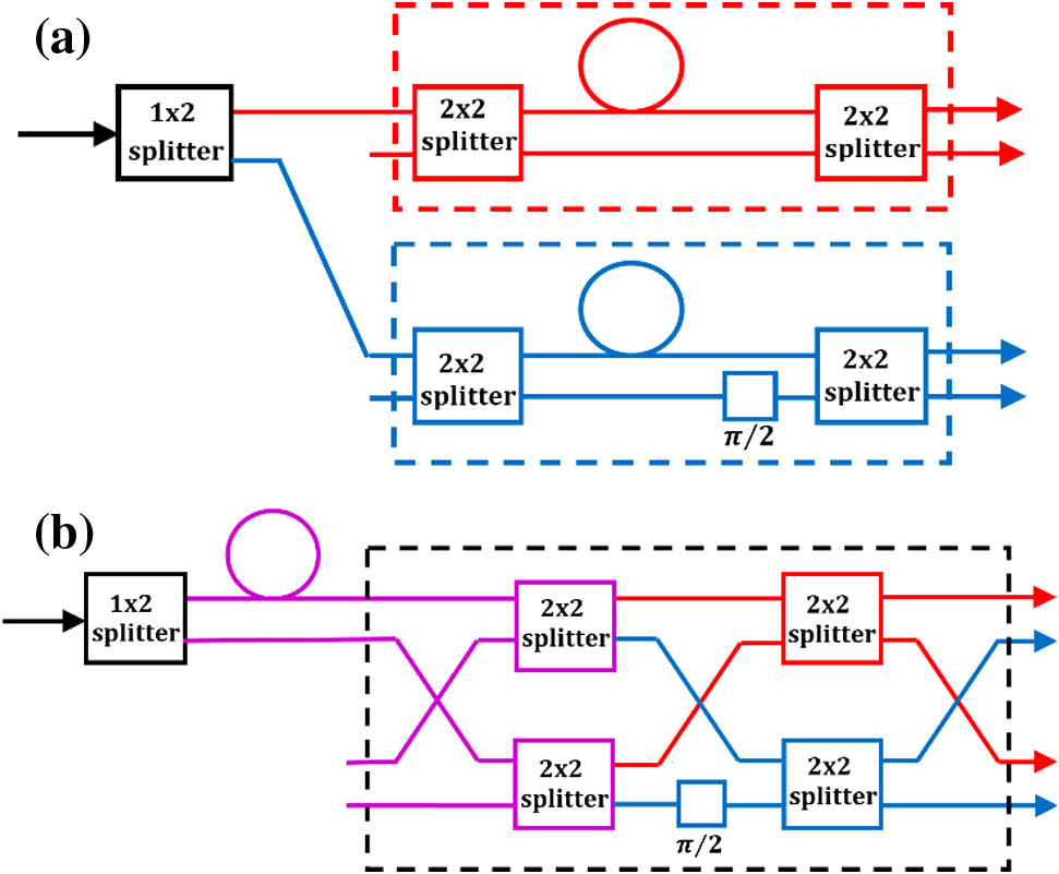
Fig. 1. (a) Schematic of a two-stage interferometer architecture consisting of two parallel 2×2 MZI. The two MZIs, including the delay lines represented by the circles, are notionally identical except for the quadrature bias of the lower (blue) MZI provided by the π/2 phase shift. (b) Rearrangement of the architecture of (a). The notionally identical arms of the two MZIs, excluding the phase shift, have been brought forward and are now shared. The dashed subsystem block is recognized as the decomposition of a 4×4 DFT into a network of four 2×2 DFT blocks and a phase-shift element.

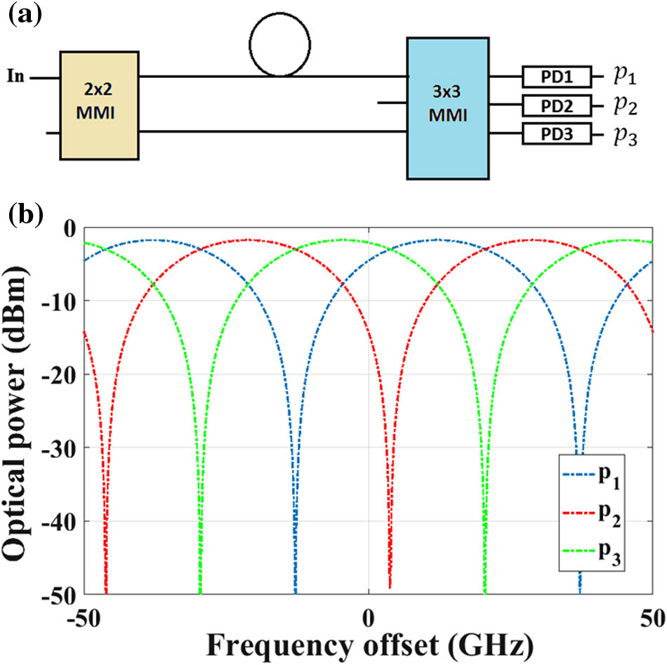
Fig. 2. (a) Schematic of a conventional wavelength meter system. (b) Ideal optical spectra of the egress ports of the output coupler.

Fig. 3. Distribution of calculated condition number of L and A and norm of A+ derived from the calibration simulations of 1000 interferometric instruments using the proposed method. Different impairment and noise settings, as listed in Table 1, correspond to different cases: (a) condition number of L, (b) condition number of A, and (c) norm of A+ belong to Case I; (d) condition number of L, (e) condition number of A, and (f) norm of A+ belong to Case II; (g) condition number of L, (h) condition number of A, and (i) norm of A+ belong to Case III; (j) condition number of L, (k) condition number of A, and (l) norm of A+ belong to Case IV; and (m) condition number of L, (n) condition number of A, and (o) norm of A+ belong to Case V.

Fig. 4. (a) Correct object samples retrieved by the conventional method and object samples retrieved using the proposed method. (b) Output port fringe pattern samples (marker) accompanied by the fitted fringe pattern (solid) provided by the proposed method. (c) Comparison between the frequency measured using the conventional and proposed methods. (d) Comparison between the residual measured and source frequency using the conventional and proposed methods. The wavelength meter simulated has an MZI architecture based on a 3×3 MMI output coupler with all components impaired. The reference frequency is 193.4 THz (wavelength 1.55 μm).

Fig. 5. Mean residual between estimated and original frequency using the (a) proposed and (b) conventional methods; standard deviation of the calculated residual between estimated and original frequency using the (c) proposed and (d) conventional methods. The reference frequency is 193.4 THz (wavelength 1.55 μm).

Fig. 6. (a) Correct object samples retrieved by the conventional method and object samples retrieved using the proposed method. (b) Comparison between the residual measured and source frequency using the conventional and proposed methods. The wavelength meter simulated has an MZI architecture based on a 4×4 MMI output coupler with all components impaired. The reference frequency is 193.4 THz (wavelength 1.55 μm).

Fig. 7. Micrograph of the fabricated on-chip wavelength meter.

Fig. 8. (a) Recorded output port intensity (markers) from the three output ports of the 3×3 MMI coupler and the fit provided by the proposed algorithm (solid). (b) Frequency offset retrieved from the power sensor data by the conventional and proposed approaches versus the original frequency. (c) Residual error in calculating the frequency over the desired frequency span. For the following figures, the test data processed are extracted from the adjacent FSR to the data used for training. (d) Recorded output port intensity (markers) from the three output ports of the 3×3 MMI coupler and the fit provided by the proposed algorithm (solid). (e) Frequency offset retrieved from the power sensor data by the conventional and proposed approaches versus the original frequency. (f) Residual error in calculating the frequency over the desired frequency span. The reference frequency is 193.4 THz (wavelength 1.55 μm).

Fig. 9. Residual error in calculating the frequency over the desired frequency span for different reference frequencies.

Table 1. Simulation Parameter for Impairment and Noise

Table 2. Simulation Parameter Applied for Operation