Gazi Mahamud Hasan, Mehedi Hasan, Peng Liu, Mohammad Rad, Eric Bernier, Trevor James Hall, "Optical wavelength meter with machine learning enhanced precision," Photonics Res. 11, 420 (2023)
Copy Citation Text
A photonic implementation of a wavelength meter typically applies an interferometer to measure the frequency-dependent phase shift provided by an optical delay line. This work shows that the information to be retrieved is encoded by a vector restricted to a circular cone within a 3D Cartesian object space. The measured data belong to the image of the object space under a linear orthogonal map. Component impairments result in broken orthogonal symmetry, but the mapping remains linear. The circular cone is retained as the object space, which suggests that the conventional conic section fitting for the wavelength meter application is a premature reduction of the object space from to . The inverse map, constructed by a learning algorithm, compensates impairments such as source intensity fluctuation and errors in delay time, coupler transmission, and photoreceiver sensitivity while being robust to noise. The simple algorithm does not require initial estimates for all parameters except for a broad bracket of the delay; further, weak nonlinearity introduced by uncertain delay can be corrected by a robust golden search algorithm. The phase-retrieval process is invariant to source power and its fluctuation. Simulations demonstrate that, to the extent that the ten parameters of the interferometer model capture all significant impairments, a precision limited only by the level of random noise is attainable. Applied to measured data collected from a fabricated wavelength meter, greater than an order of magnitude improvement in precision compared with the conventional method is achieved.
1. INTRODUCTION
Interferometric methods are extensively used in diverse applications, including inter alia optical communications coherent receiver front ends [1] and spectral monitoring [2]; Bragg grating sensor interrogation [3]; laser intensity and frequency fluctuation metrology [4,5]; and fiber optic sensing of temperature [6], pressure [7], refractive index [8], and strain [9]. Common interferometric architectures involving a Mach–Zehnder interferometer [10], Michelson interferometer [5,11], or Fabry–Perot interferometer [12] are employed to convert a phase shift provided by some sensing means to a measurable change in light intensity. Mach–Zehnder interferometers (MZIs) formed by circuits of planar waveguides and couplers are particularly attractive for photonic integration.
The fundamental principle of a wavelength meter or frequency discriminator is the use of an interferometer to measure the phase difference between the original signal and a delayed replica of the signal. The delay converts a change of frequency to a change of relative phase between the original and replica signals. The conventional MZI structure has a co-sinusoidal response to the relative phase; hence, the sensitivity to small frequency deviations varies over its period. In frequency discriminator applications, it is necessary to maintain a quadrature phase bias to maximize sensitivity and, in wavelength meter applications, the loss of precision at null and peak bias points is a concern.
To avoid this signal fading problem in passive structures, Sheem introduced an MZI architecture using couplers to provide a three-phase output [13]. Koo et al. developed a demodulation method that projects the three-phase output onto quadrature phase components from which a continuous phase is retrieved by a process involving differentiation, cross multiplication, summation, and integration [14]. Jin et al. applied least-squares estimation to the digitized quadrature components to recover the variation in amplitude and phase [15]. Todd et al. disclosed a Bragg grating sensor interrogation system that projects the digitized three-phase output onto quadrature components from which the phase is retrieved via a digital arctangent function [3]. Todd’s original method assumes an ideal coupler. Todd et al. subsequently extended the method to incorporate nonideal coupler parameters, which involves a weighted linear combination of outputs to which the digital arctangent is applied [10]. Xu et al. applied the extended approach to laser phase and frequency noise metrology [5]. The characterization of the impairments of a component in isolation is often not possible consequently; it is Todd’s original method that has become the conventional method of interferometric data processing. Wu et al. showed that the conventional approach is superior to preceding methods for a high-power signal in a severely noisy environment [16].
Sign up for Photonics Research TOC. Get the latest issue of Photonics Research delivered right to you!Sign up now
Kleijn et al. applied a nonlinear least-squares fitting procedure to calibration data provided by a MMI based MZI wavelength meter [17]. A total of 10 parameters are extracted: six coupler scattering magnitudes, three coupler phase shifts, and one delay; which enable the compensation of uncertain coupler transmission matrices, interferometer delay imbalance, and photodetector responsivity. The convergence of the fitting algorithm requires good starting points for all parameters. Moreover, the parameter estimation requires knowledge of the source power used during calibration and operation modes. The sum of the output port powers of the interferometers is used for this purpose, but this sum is only substantially independent of the measurand for small impairments.
Motivated by the Lissajous figure traced by any pair of delay interferometer outputs as the frequency is scanned, researchers have applied a curve-fitting method developed by Fitzgibbon et al. [18], which is a specific case of Bookstein’s conic-section fitting method [19], to fit an ellipse [11] or squircle [20] to extract phase-retrieval parameters from scattered data. Recently, a 90° hybrid (e.g., a MMI) based MZI has been applied to the measurement of laser frequency fluctuations [4], and Chen et al. demonstrated a parallel arrangement of MMI-based wavelength meters with waveguide delay lines engineered to relax temperature sensitivity [21].
This paper re-examines the interferometric wavelength measurement problem. An object vector composed of an in-phase, quadrature phase, and input power component emerges in the ideal case as a representation of the autocorrelation of the input sequence to a discrete Fourier transform (DFT) representing the interferometer output coupler. The vector belongs to a circular cone within an object space . Each point on the cone is sent by an orthogonal map to a vector of interferometer egress port photoreceiver outputs in an image space , . In the nonideal case, intensity fluctuations of the source, impairments of the waveguide delay line and interferometer couplers, and sensitivity errors of the photoreceiver array and noise are considered. It is found that the circular cone is retained as the fundamental object on which the data to be retrieved are located. The component impairments break the orthogonal symmetry, but the map from the cone to the image space remains linear. An information-retrieval problem is formulated for a known delay as the construction using linear algebra only of a matrix representing the linear map that minimizes the sum of the squared prediction error over a training data set. An uncertain delay introduces nonlinearity, but a few iterations of a golden search algorithm suffice to retrieve the delay parameter. The method corrects the same comprehensive set of impairments as Kleijn’s method while eliminating its deficiencies. The algorithm is simple and robust. No parameter starting points are required; only the time-delay parameter requires bracketing over a broad interval. The calibration and phase retrieval process is invariant to source power. The retrieval process is naturally invariant to source optical power fluctuations during data processing.
2. THEORY
A. Perfect Components
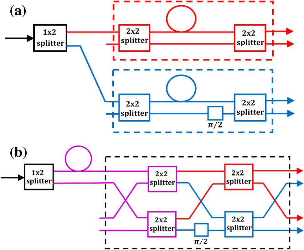
Figure 1(a) illustrates a dual MZI approach to eliminate signal fading suffered by a single MZI architecture [22]. The signal is split between two parallel MZIs that are notionally identical with the exception that one MZI is biased in quadrature relative to the other. Ideally, each MZI is lossless; consequently, the intensities of their two output ports are complementary. The difference in intensity between the two output ports of each MZI provides a signed in-phase component and a signed quadrature-phase component of the phasor that describes the interference term. It is then straightforward to recover the phase with a frequency-invariant sensitivity.
Figure 1.(a) Schematic of a two-stage interferometer architecture consisting of two parallel MZI. The two MZIs, including the delay lines represented by the circles, are notionally identical except for the quadrature bias of the lower (blue) MZI provided by the phase shift. (b) Rearrangement of the architecture of (a). The notionally identical arms of the two MZIs, excluding the phase shift, have been brought forward and are now shared. The dashed subsystem block is recognized as the decomposition of a DFT into a network of four DFT blocks and a phase-shift element.
In its improved version, as illustrated in Fig. 1(b), the sharing of a delay line between two MZIs guarantees that the two delay lines in Fig. 1(a) are identical. The network of four couplers and a phase shift is recognized as an instance of a DFT, which may be implemented alternatively using a single coupler. For example, multimode interference (MMI) couplers with a uniform split ratio have transmission matrices that are phase-permutation equivalent to a Fourier matrix.
This rearrangement provides the motivation to consider a general interferometer architecture consisting of a uniform splitter and an Fourier coupler interconnected by arms with imbalanced phase. The transmission matrix of the output coupler maps a column vector composed of the complex field amplitudes at its ingress ports to a column vector composed of the complex field amplitude at its egress ports:
Each datum is a vector with elements equal to the modulus squared of the amplitude at each egress port, which can be identified with the diagonal of the outer product which is related to the outer product by
The measured output port power vector is then given by where the basis vector has a unit element in position and zeros elsewhere. In the special case of a transmission matrix that is a Fourier matrix: where is the identity matrix. The outer product has the representation
Substituting Eq. (6) into Eq. (4) noting and collecting terms with , yields
Equation (8) is a restatement in matrix/column vector form of the familiar result that the modulus squared of the discrete Fourier transform of a sequence is equal to the discrete Fourier transform of the circular autocorrelation of the sequence. The vector is the result of summing over the trailing diagonals of . A vector of length generates nonzero trailing diagonals. The cyclic nature of the summation in Eq. (8) does not come into play if zero padding leads to . The vector may then be expressed by a total of real-valued components, which is the largest number of knowable unknowns that may be recovered from the measurement. For and unit input power, the vector takes the form where is the phase imbalance of the two arms, and are orthonormal vectors: where is the null vector representing the zero padding. The vector contains all the information to be retrieved: the in-phase term , the quadrature-phase term , and the input power appear as weights of its three orthonormal components. The phase may be extracted by introducing the real scalar coordinates and evaluating the arctangent interpreted in the four-quadrant sense. The coordinates satisfy which defines a double-napped circular cone in .
The Fourier matrix preserves the inner product so that where are the transformed basis:
Together, Eqs. (9) and (14) define a real orthogonal map such that
The transpose may be used to project the measured data onto the 3D space containing the circular cone. The image of the object under the orthogonal map also lives on a cone. The conic shape is a consequence of linearity, and the absence of deformation is a consequence of orthogonality. The invariance of the cone to rotation about its axis corresponds to a translation of the phase. The mirror symmetry in any plane containing the axis or in the plane at the origin perpendicular to the axis results in a reversal of the direction clockwise or anticlockwise of increasing phase. A specific choice of coordinate system and a calibration measurement are necessary to fix the phase origin and direction.
B. Imperfect Components
The optical system is equivalent to a parallel arrangement of copies of a single input and output port MZI terminated by photoreceivers and driven by a perfect splitter. Consequently, the measurement at a selected egress port of the output coupler is of the form where and are the complex transmissions of the paths from the input port through one or other of the interferometer arms to the selected output port, excluding the phase contributed by the delay line and scaled by a real constant to account for photoreceiver sensitivity. The impairments affect the power bias , phase origin , and amplitude of the recorded fringe patterns. The orthogonal symmetry is broken, but the map remains linear, and the circular cone is retained as the fundamental object on which the data to be retrieved are located.
C. Learning Algorithm
A linear system that maps an input to an output may be described by a matrix :
Suppose a sequence of measurements is made of pairs of inputs and outputs associated by the system, which are assembled into a collection of data known as the training set
The task is to reconstruct from . In practice, the training set is corrupted by measurement errors and noise, so the problem is reformulated as finding an that minimizes an error function defined by where denotes the Frobenius inner product. The Gâteaux derivative of evaluated on the tangent vector is given by where
Consequently, the error function is minimized by the choice
In general, is not invertible if . However, the Moore–Penrose inverse provides the minimum norm least-squares solution of Eq. (18). In practice, the system is overdetermined, which leads to the explicit expression
An individual measurement can be mapped to the object space by evaluating and its phase retrieved using , where the arctangent function is interpreted in the four-quadrant sense. However, in experiments, there is no direct object space measurement; only the frequency of the input is measured and paired with the image space measurement. The object space data are parameterized by the phase , which must be inferred from the measured frequency using; if dispersion is neglected, the relationship where is some nominal reference frequency, is the interferometer delay imbalance, and is the phase at .
The phase bias is sensitive to fabrication process variations and hence uncertain. It acts as a rotation about the axis of the circular cone on which the object samples live. The group of rotations is a subgroup of the general linear group to which belongs. Consequently, the phase bias in Eq. (26) may be dropped and its action as a rotation absorbed into .
The delay is robust to fluctuations of the ambient environment. It may be determined by design through accurate knowledge of the physical path length imbalance and the group index of the waveguide and refined by a measurement of the free-spectral range (FSR) of the interferometer. The latter may be done by applying a golden section search for the delay that minimizes the residual error given by Eq. (20) after substitution of Eq. (23).
3. RESULTS AND DISCUSSION
A. Simulation
A schematic of the conventional wavelength interrogation system considered for validation of the proposed method and the optical spectra at the three outputs are shown Figs. 2(a) and 2(b). The Virtual Photonics Inc. (VPI) software package has been used to derive these spectra. The unbalanced MZI architecture consists of a MMI input coupler and MMI output coupler with an ideal path length difference between its two arms corresponding to a free spectral range (FSR) of 50 GHz. For an ideal system, the outputs of the identical photoreceivers can be expressed as where is proportional to the input optical power and the responsivity of the photoreceivers, and
Figure 2.(a) Schematic of a conventional wavelength meter system. (b) Ideal optical spectra of the egress ports of the output coupler.
Equations (27) and (28) can be derived from Eqs. (14)–(16) with appropriate allowance for phase permutation equivalence of MMI and Fourier couplers; no adjustment of the proposed data-processing method is necessary. Impairments due to imperfect couplers, photoreceivers, and interferometer arms break the orthogonal symmetry, but the concept of the circular cone as the fundamental object remains useful since all these impairments are encompassed by the linear map . Fluctuations and noise will also be added by source power fluctuations, photoreceiver, and quantization noise. These errors are accommodated by the least-squares fit of the system map to the training set and the Moore–Penrose inverse used for data processing. The deviations from the ideal case will be small, and the port data are clearly recognisable as a poly-phase fringe pattern. The phase retrieved for a given linear map is robust to source power fluctuations, as the linearity in input power of the system ensures that the object samples lie on the cone irrespective of source power.
A MATLAB code was developed to evaluate the performance of the learning algorithm in processing data generated by a simulated wavelength meter subject to a variety of random impairments. Simulation of a wavelength meter with perturbed interferometer delay imbalance and arbitrary phase bias provides synthetic measured data for further data processing. Impairments are added to the coupler transmission matrices and to the responsivities to emulate fabrication process variations and component tolerances. A matrix represents the instrument map where large perturbation is provided by the different impairments discussed. Gaussian noise is added to emulate thermal, RIN, quantum, and quantisation noise processes that occur during measurements made during the calibration and operation phases. To elucidate the robustness of the proposed algorithm against impairments and noise, a process is considered where it is perceived that 1000 instruments are available from the same manufacturer. There will be differences from instrument to instrument; however, for a tightly controlled standard process, in practice, the variability would be a small about a static but impaired “mean” instrument. Design variations could move that mean closer to a perfect “mean” instrument. Randomized impairments representing this variability are applied in the simulation of these 1000 interferometric instruments. Impairments of the couplers are introduced by Gaussian-distributed real and imaginary parts of transmission matrix components. Table 1 lists five cases where the degree of impairment has been increased gradually by varying the symmetry-preserving and symmetry-breaking perturbation parameters of the couplers. The impairments of the delay-line delay time and photoreceiver responsivities follow a Gaussian distribution; however, their standard deviations are kept constant at and , respectively, in all these cases.
After projecting these impairments, has been generated for an individual interferometer. The instrument is then trained with an independent training set with associated additive random noise. The signal-to-noise ratio (SNR) is varied between different cases. The training set is used to estimate and refine the delay imbalance and thus obtain via the proposed learning method. The matrix can, at best, inherit the condition number of ; there is no data-processing method able to retrieve information that is not present in the data. Figure 3 depicts distributions of the condition number of , , and the norm of the Moore–Penrose inverse for all cases. It can be observed that the distributions of the condition number of are well-bounded and follow almost exactly the distributions for for all cases. For severe impairment and noise, the condition number of remains of the order of unity, which explains how the linear mapping can approximate the orthogonal mapping in the limited impairment case; consequently, the inverse of is well-conditioned and processed continuous results for the data. It is possible to generate extreme impairments resulting in singular and extreme condition numbers; however, these are outliers characterizing a poor fabrication run that has destroyed the inherent DFT phase relationship of the couplers. As these extreme cases are rare, they can be removed in practice by adopting a quality-control procedure that discards an interferometer with too severe impairment.
Figure 3.Distribution of calculated condition number of and and norm of derived from the calibration simulations of 1000 interferometric instruments using the proposed method. Different impairment and noise settings, as listed in Table 1, correspond to different cases: (a) condition number of , (b) condition number of , and (c) norm of belong to Case I; (d) condition number of , (e) condition number of , and (f) norm of belong to Case II; (g) condition number of , (h) condition number of , and (i) norm of belong to Case III; (j) condition number of , (k) condition number of , and (l) norm of belong to Case IV; and (m) condition number of , (n) condition number of , and (o) norm of belong to Case V.
Figure 3 also shows that the distributions of the norm of are also well-bounded and close to unity. From linear algebra, it can be inferred that the noise of the processed data (before calculating the arctangent) is increased by no more than the norm of the Moore–Penrose inverse of ; further, as this norm is bounded (close to unity), it can be concluded that the processed data are stable, i.e., small perturbations such as noise are not significantly magnified.
To observe the effects of additive noise in the operation phase as well, an interferometer with an arbitrary condition number is chosen to be perturbed with impairment and calibration noise setting of Case I, and the proposed method is applied. After learning, the interferometer processes a test data set. In the operation stage, additive Gaussian noise providing SNR of 30 dB has been applied. Figure 4 shows the associated simulation results. Figure 4(a) shows that the projection by the Moore–Penrose inverse of the simulated measured data [Fig. 4(b)] has an excellent match to the original object data. Likewise, the mapping of the original object space by the linear map estimated from the training data provides an excellent fit to the simulated output port fringe patterns shown in Fig. 4(b). To judge the efficacy of the proposed algorithm, the conventional method due to Todd et al., where impaired image space data are processed by the orthogonal mapping of the perfect interferometer, has also been applied [3]. It can be observed from Fig. 4(a) that the conventional method results in poor object sample estimation, which is reflected in the corresponding retrieved-frequency plot shown in Figs. 4(c) and 4(d). A substantial improvement in the accuracy of the retrieved frequency is achieved by the proposed algorithm, as shown in Figs. 4(c) and 4(d).
Figure 4.(a) Correct object samples retrieved by the conventional method and object samples retrieved using the proposed method. (b) Output port fringe pattern samples (marker) accompanied by the fitted fringe pattern (solid) provided by the proposed method. (c) Comparison between the frequency measured using the conventional and proposed methods. (d) Comparison between the residual measured and source frequency using the conventional and proposed methods. The wavelength meter simulated has an MZI architecture based on a MMI output coupler with all components impaired. The reference frequency is 193.4 THz (wavelength 1.55 μm).
To make the comparison between the proposed and conventional methods more evident, seven interferometers, after going through the impairment and learning process, are selected to have mappings with different condition numbers representative of different static impairments and calibration noise. Table 2 lists the corresponding parameters. Each interferometer processes 100 test data sets. Figure 5 shows the mean error and standard deviation of the distribution in estimating individual frequency samples of each wavelength meter. It can be observed from Figs. 5(a) and 5(c) that, even with the most severe impairment setting, the estimation error processed by the proposed approach is smaller than 0.4 GHz on average. The conventional approach cannot achieve such performance even with the least impairment and noise setting. It is evident from the mean error and standard deviation in Fig. 5(d) that small inherent impairments due to design flaw or fabrication limitation followed by noise in the learning and measurement stages limit the performance of the conventional approach and result in failure in predicting the wavelength with reliable precision.
Simulation Parameter Applied for Operation
Case
Impairment and Calibration Noise Setting
Condition Number of Chosen
Additive Noise in the Operation Stage
A
Case I
1.2456
Gaussian distribution; noise-equivalent optical power of
B
Case II
1.8982
Gaussian distribution; noise-equivalent optical power of
C
Case III
2.9186
Gaussian distribution; noise-equivalent optical power of
D
Case IV
4.4648
Gaussian distribution; noise equivalent optical power of
E
Case V
11.0627
Gaussian distribution; noise-equivalent optical power of
F
Case V
7.6899
Uniform distribution; noise-equivalent optical power of
G
Case V
10.6547
Uniform distribution; noise-equivalent optical power of
Figure 5.Mean residual between estimated and original frequency using the (a) proposed and (b) conventional methods; standard deviation of the calculated residual between estimated and original frequency using the (c) proposed and (d) conventional methods. The reference frequency is 193.4 THz (wavelength 1.55 μm).
The simulation trials confirmed that: The training and phase retrieval algorithms are invariant to static source power and phase bias. The calibration and test source powers may differ in value. The retrieved phase is naturally invariant to fluctuations from sample to sample of the test source power. The calibration process with a source power monitor is also invariant to fluctuations from sample to sample of the calibration source power.The code functions with a training set containing as few as four frequency samples providing 12 knowns to retrieve 10 unknown parameters.In the absence of additive noise, the method fully corrects all simulated impairments to machine precision provided the golden section search accuracy parameter is small enough. The loss of precision with increasing noise is graceful. The largest contributor to the loss of precision is noise in the phase-retrieval process. The loss of precision of the calibration process due to noise is reduced by the averaging over the training set. It is expected that the noise in most applications will be small () given the modest photoreceiver bandwidth requirement.
To confirm the generality of the proposed algorithm, another wavelength meter with a MMI coupler replaced by a MMI coupler has also been investigated. The resulting orthogonal map is
The conventional and proposed algorithms have been applied to the same set of impaired 4D image space data. The results shown in Figs. 6(a) and 6(b) validate the superior accuracy of the proposed algorithm in comparison with the conventional method.
Figure 6.(a) Correct object samples retrieved by the conventional method and object samples retrieved using the proposed method. (b) Comparison between the residual measured and source frequency using the conventional and proposed methods. The wavelength meter simulated has an MZI architecture based on a MMI output coupler with all components impaired. The reference frequency is 193.4 THz (wavelength 1.55 μm).
To evaluate the efficacy of the proposed data-processing method, experimental data are provided by a photonic integrated circuit wavelength meter with a MMI-based MZI circuit architecture fabricated on the CMOS-compatible photonic integration platform provided by LioniX International. Their TriPlex technology offers a variety of planar waveguide structures based on alternating silicon nitride and silicon dioxide films [23]. Among them, only the asymmetric double strip (ADS) waveguide is offered by their multiproject wafer (MPW) service. The development of an on-chip wavelength meter on was motivated by research on a compact high-resolution wideband spectrometer [24]. To meet the specifications such as low loss, low dispersion, resolution, whole C band operation, and compact size for the spectrometer, ADS technology on was chosen as the most suitable option. Figure 7 shows the micrograph of the fabricated circuit. The MZI architecture consists of a Y-junction as the input coupler and a MMI as the output coupler with a path length difference between its arms of 3393 μm. The associated FSR for the ADS waveguide is at the reference wavelength 1.55 μm (193.4 THz). Each input and output waveguide is terminated via a spot size converter (SSC) and an attached optical fibre which are not shown in Fig. 7. The ADS waveguide is optimized for TE mode propagation; thus, polarization-maintaining fibers with principal axes aligned with the chip are employed. A tunable laser (Agilent 81680A) capable of tuning over the whole C-band with 3 pm wavelength step is used as the optical input. The input power is fixed at 0 dBm. The wavelength response of the circuit is measured for a desired wavelength span around 1.55 μm. The output is detected by an optical power sensor (Agilent 81632A) and recorded by a light-wave measurement system (Agilent 8164A). The optical spectral data are collected and processed off-line by the proposed data-processing method. The experiment has been conducted in a centrally temperature-controlled laboratory environment.
Figure 7.Micrograph of the fabricated on-chip wavelength meter.
Figures 8(a)–8(c) depict the experimental results associated with a frequency span of one FSR with center vacuum wavelength 1550 nm. The learning algorithm is independent of the choice of training set center wavelength or number of FSRs spanned. Once a training set is chosen, the linear mapping is optimized for the wavelength span bounded by that set.
Figure 8.(a) Recorded output port intensity (markers) from the three output ports of the MMI coupler and the fit provided by the proposed algorithm (solid). (b) Frequency offset retrieved from the power sensor data by the conventional and proposed approaches versus the original frequency. (c) Residual error in calculating the frequency over the desired frequency span. For the following figures, the test data processed are extracted from the adjacent FSR to the data used for training. (d) Recorded output port intensity (markers) from the three output ports of the MMI coupler and the fit provided by the proposed algorithm (solid). (e) Frequency offset retrieved from the power sensor data by the conventional and proposed approaches versus the original frequency. (f) Residual error in calculating the frequency over the desired frequency span. The reference frequency is 193.4 THz (wavelength 1.55 μm).
The raw data collected from the three output ports of the MMI coupler are shown by the markers in Fig. 8(a). An excellent fit is provided by shown by the solid line fringe pattern in Fig. 8(a). Figure 8(b) depicts an almost linear relationship between the original frequency recorded by the power sensor and the measured frequency; the residual error is limited to . It can be observed in Fig. 8(c) that the prediction of the conventional method can deviate significantly from the original frequency; the maximum residual error observed over the FSR is . It is a realistic assumption that the wavelength estimation will be performed over the same span as the training data; thus, has already been calculated. To demonstrate the generalization ability of the learning algorithm, the linear mapping constructed using the training set over the FSR centered at wavelength 1550 nm is used to retrieve the frequency using test data over an adjacent FSR. Figures 8(d)–8(f) show that the maximum residual error of the proposed approach increases only slightly to , which may be expected, as is not optimized for this test data set but remains substantially superior in precision compared with the conventional method.
Figure 9 shows the frequency estimation error observed for a total span of 950 GHz. Recorded data contained in one FSR around the center frequency depicted in Fig. 5 are taken as the training set. After each calibration, recorded test data aligned to the respective FSR are processed by the system. It can be observed that, over the total 950 GHz span, the residual error is limited to .
Figure 9.Residual error in calculating the frequency over the desired frequency span for different reference frequencies.
Although the precision achieved experimentally is over one order of magnitude greater than the conventional method, it is not as great as that achieved in simulations where precision is only limited by noise. This indicates that performance is limited by weak impairment mechanisms not captured by the model. Observations point to phenomena involving reflections and a mixed polarization state to explain the current limit to the precision. A learning algorithm based on a model (a priori knowledge) with numerous parameters risks overfitting the data at the expense of generalization ability. The current model is parsimonious and comprehensive. Consequently, rather than increasing the complexity of the model, it is preferable that the interferometer meets the assumptions of the model. If sufficient care is taken to avoid spurious reflections and to maintain the state of polarization by improved component and circuit designs, the only deviations would be due to the finite bandwidth of the components and the dispersion of the waveguide. It is only errors of the cone inferred by the data processor from a data set that will propagate to subsequent phase measurements.
Fluctuations in the calibration source power during the training set collection can misplace data off the circular cone and thereby impair construction of the linear map leading to error in the phase retrieval. The resolution of this issue, if significant, is to monitor the calibration source power to correctly scale the length of each object vector sample. For , the input splitter may be replaced by a input coupler. This has the merit of a symmetric architecture more robust to fabrication process variations, and the otherwise unused central egress port of the input coupler may monitor the input power. It is only necessary that the measurement is proportional to the input power; a precise value of responsivity is not required.
To evaluate long-term stability, an experiment was performed in which training and test data sets were collected with time intervals of several hours, and the results showed significant long-term stability. The prototype featured no input power monitoring, temperature sensor, or control mechanism. Thus, an experimental study to assess long-term stability with proper temperature control and input power monitoring is left to a future endeavor. Nevertheless, it is expected that the principal source of drift is the temperature sensitivity of the bias phase of the interferometer. This can be corrected by collecting training set data over a range of temperatures as measured by an on-chip temperature sensor. It is expected that the differences between estimated linear maps corresponding to different temperatures will be a rotation. Moreover, the rotation angle or, equivalently, the phase bias is expected to be linear in the temperature range [21]. Consequently, knowledge of the temperature coefficient is enough to compensate for temperature drift.
4. CONCLUSION
In conclusion, this work has analyzed an interferometer with three or more polyphase outputs. The theoretical analysis has informed the formulation of a machine learning and data-processing method that corrects for imperfections of the interferometer components. The simulations demonstrate that a precision limited only by the level of random noise is attainable to the extent the model of the interferometer captures all significant impairments. The experimental observations using an MZI-based wavelength meter demonstrate an order of magnitude reduction in frequency estimation error compared with the conventional method. The maximum residual error is limited to over a 50 GHz FSR.
Acknowledgment
Acknowledgment. The authors acknowledge Huawei Technologies Canada for its support through a project contract. T. J. Hall is grateful to the University of Ottawa for its support of a University Research Chair. G. M. Hasan acknowledges the Ontario Student Assistance Program for its support through the Ontario Graduate Scholarship. G. M. Hasan is also grateful to the University of Ottawa for its support through an international admission scholarship.
[15] W. Jin, D. Walsh, D. Uttamchandani, B. Culshaw. A digital technique for passive demodulation in a fiber optic homodyne. Proceedings 1st European Conference on Smart Structures and Materials, 1777, 57(1992).
[21] L. Chen, C. Doerr, S. Liu, L. Chen, M. Xu. Silicon-based integrated broadband wavelength-meter with low temperature sensitivity. Optical Fiber Communication Conference, M1C-3(2020).
Gazi Mahamud Hasan, Mehedi Hasan, Peng Liu, Mohammad Rad, Eric Bernier, Trevor James Hall, "Optical wavelength meter with machine learning enhanced precision," Photonics Res. 11, 420 (2023)