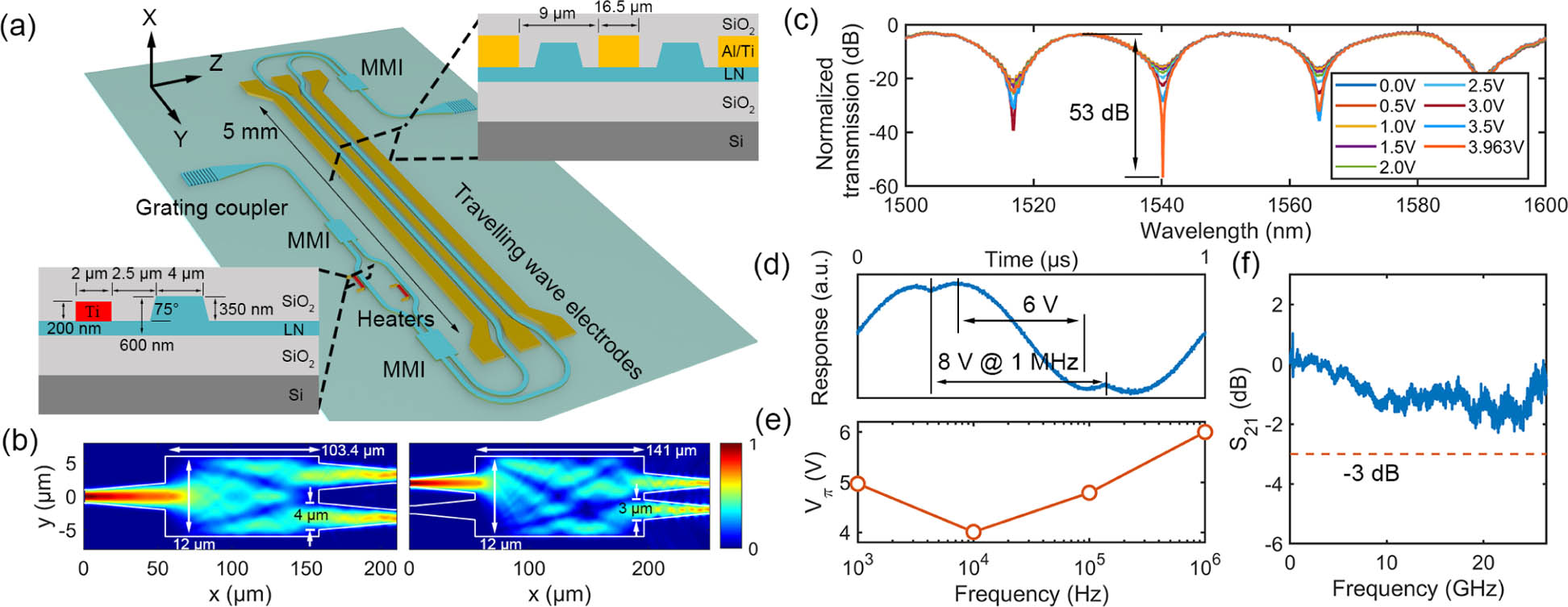
Fig. 1. (a) Schematic of the cascaded-MZI EOM. Insets: cross-section views of the thermo-optic structure in the first MZI and the electro-optical structure in the second (modulation) MZI. (b) Electric field magnitude distributions of the 1×2 MMI (left) and 2×2 MMI (right) used in the modulator. (c) Measured transmission spectra for different DC voltages applied to the heater. (d) EO response under triangular-wave driving at 1-MHz frequency. (e) Measured Vπ versus driving frequency. (f) Measured EO bandwidth (S21) of the EOM.

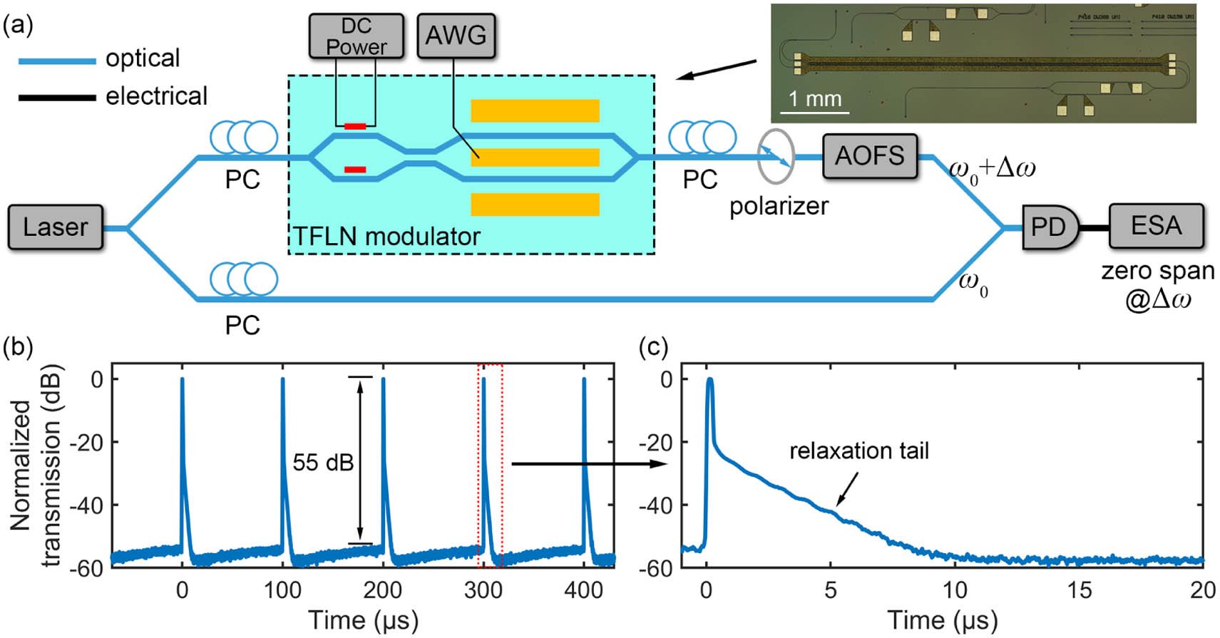
Fig. 2. (a) Schematic of the self-heterodyne measurement setup. AWG, arbitrary waveform generator; PC, polarization controller; AOFS, acousto-optic frequency shifter; PD, photodetector; ESA, electrical spectrum analyzer. Inset: micrograph of the TFLN EOM. (b) Measured high-ER waveform of modulated optical pulse train. (c) Zoom-in waveform of the red dashed box in (b).

Fig. 3. (a) Measured current versus voltage for the upper-SiO2-TFLN and the lower- SiO2-Si interfaces using the probing methods on the left. (b) Proposed electrical model with three interface conductivities. (c) Experimental step response of the EOM and simulated responses with σ2, σ2×10, and σ2×0.1. (d) Simulated temporal evolutions of horizontal electric field at waveguide center [red triangle marked in (b)] driven by pulses of 200-ns, 400-ns, and 600-ns durations. (e) Simulated electric field distributions at the moments I–IV marked in (d). (f) Experimental and simulated EOM response driven by pulses of 200-ns, 400-ns and 600-ns durations.

Fig. 4. (a) Modified driving signals (upper panel) and corresponding recorded optical pulse waveforms (lower panel) in the process of relaxation tail suppression. (b) Pulse train waveform (200-ns duration and 10-kHz repetition) after complete suppression of tail.

Fig. 5. (a) Schematic of ϕ-OTDR system. The symbol “s” represents 10-m fiber length difference for 20-m delay. DAQ, data acquisition. Inset: photograph of the packaged TFLN EOM. (b) Demodulated phase change signal (black dots) and fitted sinusoidal waveform (blue curve). (c) PSD of the phase change signal from 100 Hz to 2100 Hz. (d) Averaged PSD near vibration frequency along the fiber. Inset: zoom-in PSD in linear scale around the PZT position.

Fig. 6. (a) Probability density distributions of measured spatial crosstalk noise (SCN) for different ERs of the EOM. (b) SCN and noise floor for the maximum probability densities on the fitted curves dependent on ER. (c) Averaged PSD near vibration frequency along the fiber in tailed (orange) and sharp (blue) probe pulses at 10-kHz repetition. The green circle marks the signal position. (d) Probability density distributions of SCN after PZT between 1060 m and 1400 m in tailed (orange) and sharp (blue) probe pulse at 10-kHz repetition. (e) Averaged PSD near vibration frequency along the fiber in tailed (orange) and sharp (blue) probe pulse at 50-kHz repetition. The green circle marks the signal position. (f) Probability density distributions of SCN after PZT in tailed (orange) and sharp (blue) probe pulse at 50-kHz repetition.

Fig. 7. Simulated propagation loss and VπL versus gap size with the electrodes (a) beside the waveguide and (b) on silica cladding.

Fig. 8. (a) Simulated horizontal electric field at the TFLN waveguide center [red triangle marked in Fig. 3(b)] driven by triangular signal at frequencies of 1 kHz, 10 kHz, 100 kHz, and 1 MHz. (b) Experimental and simulated Vπ against frequency.

Fig. 9. (a) Illustration of the coupling between the LP01 mode in fiber and TE1 mode in waveguide. (b) Pulse waveforms with different ERs induced by alignment offset. (c) Measured pulse peak and valley transmissions with simulated coupling efficiencies of TE0 mode and TE1 mode to LP01 mode of fiber. The simulated efficiency is normalized to the maximum transmission of pulse peak or valley.

Table 1. Electric Parameters Used in Simulation