
Qiming Li, Jieji Ren, Xiaohan Pei, Mingjun Ren, Limin Zhu, Xinquan Zhang. High-Accuracy Point Cloud Matching Algorithm for Weak-Texture Surface Based on Multi-Modal Data Cooperation[J]. Acta Optica Sinica, 2022, 42(8): 0810001
- Acta Optica Sinica
- Vol. 42, Issue 8, 0810001 (2022)
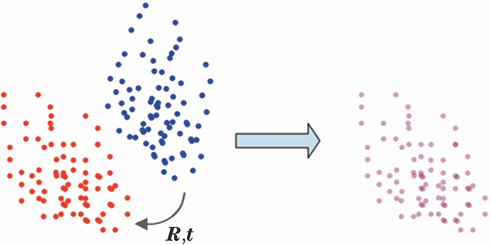
Fig. 1. Schematic diagram of ICP algorithm
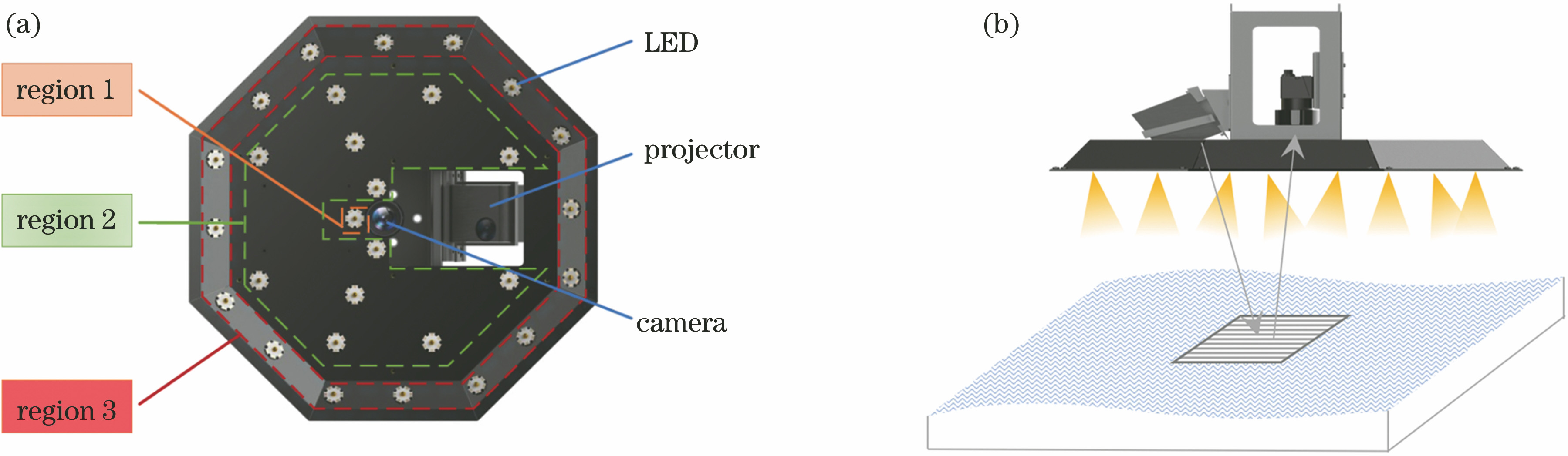
Fig. 2. Schematic diagram of compound sensor system. (a) Upward view; (b) front view
Fig. 3. Flow chart of proposed algorithm
Fig. 4. Relationship of arbitrary normal vector with its k nearest normal vectors
Fig. 5. Relationship between positions of arbitrary point and center of gravity in neighborhood
Fig. 6. Schematic diagram of weak-texture surface. (a) Three-dimensional graph of surface; (b) weak-texture graph
Fig. 7. Registration results of different algorithms. (a) Unregistered image; (b) ground-truth image; (c) ICP algorithm; (d) IRLS-ICP algorithm; (e) NICP algorithm; (f) proposed algorithm
Fig. 8. Comparison of reconstruction indicators. (a) Comparison of RMSE; (b) comparison of PV value
Fig. 9. Two-dimensional graphs of surfaces with different periods
Fig. 10. Experimental results of surfaces with different curvatures
Fig. 11. Overall diagram of experimental equipments
Fig. 12. Initial positions of point clouds. (a) Initial position of two adjacent point clouds; (b) initial position of overlapping area of point clouds
Fig. 13. Registration results for overlapping areas of point clouds. (a) ICP algorithm; (b) IRLS-ICP algorithm; (c) NICP algorithm; (d) proposed algorithm
|
Table 1. Relationship between σn and measurement error of normal vector angle
|
Table 2. Comparison of registration results

Set citation alerts for the article
Please enter your email address
© Copyright 2018-2021 | Chinese Laser Press. All Rights Reserved 沪ICP备15018463号-20