• Advanced Photonics
  • Vol. 5, Issue 1, 016005 (2023)
Valeria Cimini1, Mauro Valeri1, Emanuele Polino1, Simone Piacentini2, Francesco Ceccarelli2, Giacomo Corrielli2, Nicolò Spagnolo1, Roberto Osellame2, and Fabio Sciarrino1、*
Author Affiliations
  • 1Sapienza Università di Roma, Dipartimento di Fisica, Roma, Italy
  • 2Istituto di Fotonica e Nanotecnologie, Consiglio Nazionale delle Ricerche, Milano, Italy
  • show less
    DOI: 10.1117/1.AP.5.1.016005 Cite this Article Set citation alerts
    Valeria Cimini, Mauro Valeri, Emanuele Polino, Simone Piacentini, Francesco Ceccarelli, Giacomo Corrielli, Nicolò Spagnolo, Roberto Osellame, Fabio Sciarrino. Deep reinforcement learning for quantum multiparameter estimation[J]. Advanced Photonics, 2023, 5(1): 016005 Copy Citation Text show less
    (a) Generic multiparameter estimation problem fully managed by artificial intelligence processes. Quantum probes evolve through the investigated system and consequently their state changes depending on ϕ. Both the single-measurement update and the setting of control parameters c are done via machine-learning algorithms to optimize the information extracted per probe. (b) Sketch of the implemented protocol. A limited number of quantum probe states are fed into the sensor treated as a black box. A grid of measurement results is collected to train an NN, which learns the posterior probability distribution associated with the single-measurement Bayesian update. Such distribution is used to define the reward of an RL agent who sets the control phases on the black-box device.
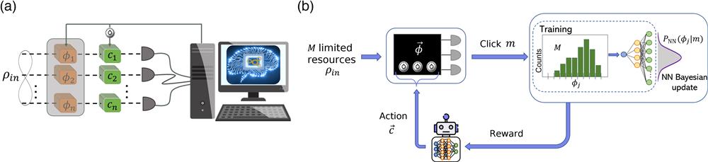
    Fig. 1. (a) Generic multiparameter estimation problem fully managed by artificial intelligence processes. Quantum probes evolve through the investigated system and consequently their state changes depending on ϕ. Both the single-measurement update and the setting of control parameters c are done via machine-learning algorithms to optimize the information extracted per probe. (b) Sketch of the implemented protocol. A limited number of quantum probe states are fed into the sensor treated as a black box. A grid of measurement results is collected to train an NN, which learns the posterior probability distribution associated with the single-measurement Bayesian update. Such distribution is used to define the reward of an RL agent who sets the control phases on the black-box device.
    Single-phase estimation in a Mach–Zehnder interferometer. (a) Averaged quadratic loss as a function of the number of probes N, computed over 30 repetitions of 100 phase values of φ∈[0,π]. The results are obtained setting the control phase to zero. We compare the results obtained when having the full knowledge of the outcome probabilities (green line), with the ones achieved using the NN-reconstructed single-measurement posterior probability (blue line) and the ones resulting from approximating the lHd of the system with the occurence frequencies (yellow line), both retrieved performing r=10 measurements for each of the Nφ=100 grid points. In the inset, we report the ratio among the average Qloss achieved with the NN and the one retrieved using the lHd for ideal (blue) and noisy (purple) conditions. We compare the results with V=0.8, changing the number of measurements r in the training set. (b) lHd functions relative to the two possible measurements outcomes reconstructed via the NN on the left and with the standard calibration procedure on the right with r=10 and Nφ=100 in the π interval. The continuous lines represent P(d|φ), for d=0 (blue) and d=1 (red). (c) Averaged quadratic loss, as a function of the number of probes N, computed over 30 repetitions of 100 phase values of φ∈[ϵ,2π−ϵ]. Results obtained with the lHd and the NN update (reported in green and blue, respectively) when estimating φ∈[ϵ,π−ϵ] without feedbacks (light green and light blue lines) and applying random feedback after each probe (green and blue lines). The shaded area in the plots represents the interval of one standard deviation, whereas the dashed black line is the SNL=1/N. (d) lHd functions relative to the two possible measurements outcomes reconstructed via the NN obtained for r=1000 and Nφ=200 in the 2π interval, for d=0 (blue) and d=1 (red). On the right is reported the posterior NN probability reconstructed after 20 probe states were measured. As discussed in the main text, due to the nonmonotoncity of the output probabilities in the considered phase interval, the posterior shows two peaks, and this makes it necessary to use different feedback. The black line represents the true value of φ.
    Fig. 2. Single-phase estimation in a Mach–Zehnder interferometer. (a) Averaged quadratic loss as a function of the number of probes N, computed over 30 repetitions of 100 phase values of φ[0,π]. The results are obtained setting the control phase to zero. We compare the results obtained when having the full knowledge of the outcome probabilities (green line), with the ones achieved using the NN-reconstructed single-measurement posterior probability (blue line) and the ones resulting from approximating the lHd of the system with the occurence frequencies (yellow line), both retrieved performing r=10 measurements for each of the Nφ=100 grid points. In the inset, we report the ratio among the average Qloss achieved with the NN and the one retrieved using the lHd for ideal (blue) and noisy (purple) conditions. We compare the results with V=0.8, changing the number of measurements r in the training set. (b) lHd functions relative to the two possible measurements outcomes reconstructed via the NN on the left and with the standard calibration procedure on the right with r=10 and Nφ=100 in the π interval. The continuous lines represent P(d|φ), for d=0 (blue) and d=1 (red). (c) Averaged quadratic loss, as a function of the number of probes N, computed over 30 repetitions of 100 phase values of φ[ϵ,2πϵ]. Results obtained with the lHd and the NN update (reported in green and blue, respectively) when estimating φ[ϵ,πϵ] without feedbacks (light green and light blue lines) and applying random feedback after each probe (green and blue lines). The shaded area in the plots represents the interval of one standard deviation, whereas the dashed black line is the SNL=1/N. (d) lHd functions relative to the two possible measurements outcomes reconstructed via the NN obtained for r=1000 and Nφ=200 in the 2π interval, for d=0 (blue) and d=1 (red). On the right is reported the posterior NN probability reconstructed after 20 probe states were measured. As discussed in the main text, due to the nonmonotoncity of the output probabilities in the considered phase interval, the posterior shows two peaks, and this makes it necessary to use different feedback. The black line represents the true value of φ.
    Scheme of the integrated photonic phase sensor. The device consists in a four-arm interferometer with the possibility of estimating three optical phases adjusting three relative phase feedbacks through thermo-optic effects. Two-photon states are injected at the device input and both the Bayesian update and the choice of the optimal feedback are done through ML-based protocols trained directly on measurement outcomes.
    Fig. 3. Scheme of the integrated photonic phase sensor. The device consists in a four-arm interferometer with the possibility of estimating three optical phases adjusting three relative phase feedbacks through thermo-optic effects. Two-photon states are injected at the device input and both the Bayesian update and the choice of the optimal feedback are done through ML-based protocols trained directly on measurement outcomes.
    Experimental posterior probability distributions reconstructed by the NN. The points on the three axes correspond to the Nϕ3=8000 grid points measured, while the color indicates the value of the probability. Only half of the 10 possible probabilities are reported here: in particular, the probabilities relative to d=1,3,5,7, and 10 are shown. In the second row, we have reported three slices, of the corresponding above probability, obtained fixing the value of one phase to zero to give more insight into the probabilities structure.
    Fig. 4. Experimental posterior probability distributions reconstructed by the NN. The points on the three axes correspond to the Nϕ3=8000 grid points measured, while the color indicates the value of the probability. Only half of the 10 possible probabilities are reported here: in particular, the probabilities relative to d=1,3,5,7,and10 are shown. In the second row, we have reported three slices, of the corresponding above probability, obtained fixing the value of one phase to zero to give more insight into the probabilities structure.
    Estimate of ϕ=[0.6,1.7,2.5] rad retrieved applying the standard Bayesian estimation using the lHd of the ideal device and optimizing the control feedbacks with the RL agent. (a) The blue line represents the prior distribution, while the orange, green, and red lines are the reconstructed posterior probabilities for the first, second, and third phases, respectively. (b) Estimated values as a function of the number of probes. Continuous lines represent the average over 30 repetitions, whereas the shaded area is the interval of one standard deviation.
    Fig. 5. Estimate of ϕ=[0.6,1.7,2.5] rad retrieved applying the standard Bayesian estimation using the lHd of the ideal device and optimizing the control feedbacks with the RL agent. (a) The blue line represents the prior distribution, while the orange, green, and red lines are the reconstructed posterior probabilities for the first, second, and third phases, respectively. (b) Estimated values as a function of the number of probes. Continuous lines represent the average over 30 repetitions, whereas the shaded area is the interval of one standard deviation.
    Three-phase estimation in a four-arm interferometer. Achieved Qlosses [Eq. (10)] averaged over 100 different triplets of phases in the interval (0,π] as a function of the number of probes. The shaded area represents the standard deviation from the mean values. (a) Performance of the ideal device obtained when the explicit model is used for the Bayesian estimation. The orange line represents the mean over all the 30 repetitions for each of the 100 parameters inspected, whereas the red line is the median over the different repetitions. The dashed line is the QCRB, relative to the mean, that for our device is 2.5/N. (b) Average over 100 triplets of phases of the median Qloss computed over 30 repetitions of the estimation protocol. Comparison with the results obtained when substituting the Bayesian updated through the explicit posterior (red line) with the one reconstructed by an NN trained on simulated data (magenta line). The blue line represents instead the performance achieved applying random feedback instead of the ones found by the RL agent. (c) Simulation on the ideal device changing the number of grid points Nϕ in the training of the Bayesian NN. Since the training for such simulations has been done in the restricted interval [0,π], here we limit the possible applied feedback to satisfy the condition ϕtrue+c∈(0,π]. The dashed lines correspond to the sensitivity saturation values given the considered discretization. (d) Experimental results achieved with the Bayesian NN update and the RL optimization algorithm (magenta points), when the latter is substituted by a random choice of feedback (blue points) and when the Bayesian update is done approximating the lHd with the occurrence frequencies (green points). Error bars represent the standard deviation of the averaged Qlosses. The magenta line shows the performance obtained with simulation done using the lHd function of the real device; it is shown as a reference.
    Fig. 6. Three-phase estimation in a four-arm interferometer. Achieved Qlosses [Eq. (10)] averaged over 100 different triplets of phases in the interval (0,π] as a function of the number of probes. The shaded area represents the standard deviation from the mean values. (a) Performance of the ideal device obtained when the explicit model is used for the Bayesian estimation. The orange line represents the mean over all the 30 repetitions for each of the 100 parameters inspected, whereas the red line is the median over the different repetitions. The dashed line is the QCRB, relative to the mean, that for our device is 2.5/N. (b) Average over 100 triplets of phases of the median Qloss computed over 30 repetitions of the estimation protocol. Comparison with the results obtained when substituting the Bayesian updated through the explicit posterior (red line) with the one reconstructed by an NN trained on simulated data (magenta line). The blue line represents instead the performance achieved applying random feedback instead of the ones found by the RL agent. (c) Simulation on the ideal device changing the number of grid points Nϕ in the training of the Bayesian NN. Since the training for such simulations has been done in the restricted interval [0,π], here we limit the possible applied feedback to satisfy the condition ϕtrue+c(0,π]. The dashed lines correspond to the sensitivity saturation values given the considered discretization. (d) Experimental results achieved with the Bayesian NN update and the RL optimization algorithm (magenta points), when the latter is substituted by a random choice of feedback (blue points) and when the Bayesian update is done approximating the lHd with the occurrence frequencies (green points). Error bars represent the standard deviation of the averaged Qlosses. The magenta line shows the performance obtained with simulation done using the lHd function of the real device; it is shown as a reference.
    Valeria Cimini, Mauro Valeri, Emanuele Polino, Simone Piacentini, Francesco Ceccarelli, Giacomo Corrielli, Nicolò Spagnolo, Roberto Osellame, Fabio Sciarrino. Deep reinforcement learning for quantum multiparameter estimation[J]. Advanced Photonics, 2023, 5(1): 016005
    Download Citation