Multiple parameter estimation is an essential task for both fundamental science and applications. For this reason, developing strategies and devices able to perform measurements with the smallest uncertainty has become a research branch of particular interest for various fields. It is known that the achievement of the ultimate precision bounds is possible only by exploiting quantum resources.1 Indeed, nowadays, quantum sensors2^,3 represent one of the most promising applications of quantum-enhanced technologies, and they are already employed for different applications, from imaging4 and biological sensing5 to gravitational wave detection.6^,7 The highest measurement precision achievable depends on the available resources; therefore, the main focus of most quantum metrology investigations relies on the optimization of such probe states and, successively, of the performed measurements to attain such limits.8^,9 However, in a real scenario, the number of quantum resources is always limited and not all the desired probe states can be prepared. It follows that, in a limited-resource regime, operating the device at its optimal working point and employing optimized control strategies10^–12 for achieving the highest estimation precision becomes crucial. The identification of such optimal feedbacks is far from being trivial in particular for quantum systems of increasing complexity and dimensions and for multiparameter estimation problems. Usually, the employed optimization algorithms are extremely time-consuming, since they have to be computed after each measurement outcome and, more importantly, they rely on the knowledge of the device’s physical model. One of the most employed methods, which assures the convergence to the ultimate precision bound, is to update the knowledge on the parameter posterior distribution through the Bayes rule after the use of each resource.13^–17 Therefore, adaptive methods generally require a precise characterization of the operation of the employed system in order to update properly the knowledge on the investigated parameters at each step of the protocol. Such requirement is still the bottleneck for the application of optimal adaptive protocols in most quantum sensing applications. A practical model-free alternative to Bayesian update combined with a computationally feasible optimization algorithm for the identification of optimal feedback is thus desirable.

In this work, we simultaneously overcome these fundamental challenges by developing a deep reinforcement learning (RL) protocol, which combines an RL agent with a deep neural network (NN), in an actual noisy multiparameter estimation experiment, where the control feedback is efficiently chosen by an intelligent agent that does not rely on any explicit hardware model. All the NN training is performed on experimental data; therefore, no additional information besides the one extracted directly from the accessible measurements is required. With this approach, we first demonstrate the convergence to the ultimate precision bound in the single-parameter estimation scenario, and then we experimentally prove to outperform standard calibration strategies, exploiting quantum resources in the limited data regime, for the simultaneous estimation of three optical phases in a state-of-the-art integrated photonic quantum sensor. The achievement of such good estimation performance is granted by the choice of the control feedback performed by a learning agent, whose reward depends on the updated knowledge of the parameters after each step of the estimation protocol. Crucially, in our work, the Bayesian update is obtained by a previously trained deep NN; therefore, it is not required at any step of the system model. With this approach, we are able to experimentally prove the validity of a model-free optimization for parameter estimation problems, opening the way to fully artificial intelligence-based quantum metrology.

To prove the validity of our approach, we start investigating the performance of a single-parameter estimation on a test-bed system, extending the protocol developed in Ref. 18 to the adaptive framework, training an NN for Bayesian update. We then generalize such an algorithm for multiparameter estimation problems using a sequential Monte Carlo (SMC) technique for the computation of the Bayesian probabilities and we combine it with an RL agent necessary to achieve good estimation precision in more complex systems. Finally, we prove experimentally the effectiveness of the combination of a deep NN for Bayesian update with an RL agent that chooses the optimal controls on an actual multiparameter photonic quantum sensor.

The demonstrated methodology and platform will arguably have a beneficial impact over several research areas where the development of integrated photonics in the quantum regime represents a fundamental tool. An example is biosensing performed at the quantum level.19^–22 Other promising directions are quantum communication and computation tasks (in this field, integrated quantum photonics is also expanding23), where the compensation of errors, the synchronization of networks, or algorithm subroutine can be performed with adaptive phase estimation protocols. In general, our work will be of importance for all those integrated photonic tasks where fully automated calibration and optimization can be necessary for their operations.

Machine learning (ML) represents a powerful alternative to the need for developing a model describing the system behavior; for this reason, its use in the most varied research fields is spreading.24^,25 Such techniques are particularly effective when applied to the study of quantum systems that usually live in a high-dimensional space and their characterization turns out to be a computationally hard task to solve, requiring the analysis of a huge amount of data.26^,27 Different supervised and unsupervised learning algorithms have been applied to solve efficiently quantum many-body problems,28 reconstruct the density matrix of high-dimensional quantum systems,29 and even to design new quantum experiments30^–34 and discover new physical concepts.35^,36 Their application to the metrology and sensing fields fosters the idea of self-calibrated quantum sensors not relying on explicit knowledge of the model describing the device operation37^–39 and retrieving Hamiltonian parameters directly from experimental data.40 As an example, Nolan et al.18 reformulated the parameter estimation problem as a classification task to overcome the calibration requirements needed from Bayesian estimation.

The term ML refers to a huge class of algorithms sharing one common feature: the ability to extrapolate some kind of knowledge directly from the data. These algorithms are then subdivided into three macroareas: supervised learning, unsupervised learning, and RL.41^,42 Although the first two kinds of algorithms have the purpose of inferring the structure relating labeled or unlabeled data, the latter refers to algorithms developed to control the dynamics of a system. This is done through a model-free feedback-based method where an intelligent agent learns to perform tasks in a defined environment, depending on the reward it receives. The purpose of the agent is to find the optimal series of actions in response to the changing state of the environment, which maximizes its reward. After the agent has been sufficiently trained, it has been demonstrated that it can beat humans in several tasks, for example, in playing games such as Go.43 When RL algorithms are combined with the output of NNs, we can speak of deep RL.44

Very recently, the use of RL algorithms has proven to be a powerful resource. Indeed, they have been deployed in different numerical works for quantum systems control,45^–49 for finding the optimal feedback in parameter estimation tasks enhancing the sensor dynamics,50^–53 and for Hamiltonian learning.26^,54^,55 Interestingly, Fiderer et al.56 developed an RL method to create efficient experiment-design heuristics for Bayesian quantum estimation, gaining a great advantage over the extremely slow previously developed algorithms.57^,58 However, these works still rely either on the full knowledge of the system’s quantum state or on the explicit likelihood (lHd) function describing the system output probabilities. Also for this reason, until now, their application has been demonstrated mostly through theoretical simulations.

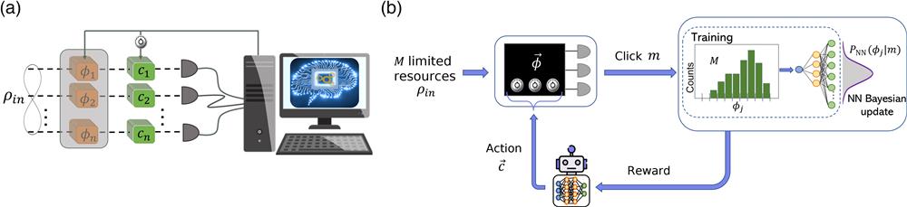
A generalization and extension of such ML approaches are thus necessary for handling realistic metrological processes over their whole spectrum. Here we develop and test experimentally a protocol fully based on artificial intelligence, which governs a real noisy sensor, from learning how to update the Bayesian belief over the system dynamics, to the optimal choice of actions to be performed in order to speed up the estimation performance. In order to do so, we extended and combined the two aforementioned ML algorithms in Refs. 18 and 56 to demonstrate a black-box adaptive multiparameter quantum estimation protocol in a real photonic device, where the unknown parameters are the relative phase shifts between the arms of an interferometer (see Fig. 1).

The purpose of estimation protocols is to retrieve the values of a vector of parameters ϕ through the measurement with a previously prepared probe. When the probe state interacts with the investigated system, its state changes depending on the parameters’ vector ϕ; therefore, the measurement of the state of the probe after such an evolution allows us to give an estimate of the parameters. To correctly assess their values, it is necessary to reconstruct the detection probabilities of all the possible measurement outcomes. Bayesian protocols use the measurement results to update the a priori knowledge p(ϕ) on the parameters under investigation retrieving the posterior probability distribution through the Bayes’s rule: P(ϕ|d)=P(d|ϕ)p(ϕ)p(d).(1)Here P(d|ϕ) is the lHd function describing the probability of obtaining a certain measurement outcome d, which can be retrieved from the Born’s rule as follows: P(d|ϕ)=Tr[Πdρ(ϕ)],(2)where {Πd} represents the complete set of positive-operator-valued measurements among the possible D output results, i.e., d∈{d1,…,dD}. Knowing the explicit model of the system under study, it is then possible to compute the mean of the posterior probability P(ϕ|d), reconstructed after sending N probes, from which it is possible to retrieve the estimate ϕ^ of the investigated parameters as follows: ϕ^=∫ϕP(ϕ|d)dϕ.(3)

To overcome the need for reconstructing the explicit model of the detection probabilities, we train a feed-forward NN for the reconstruction of such posterior probability distributions. The network requires the discretization of the continuous parameters’ space in order to treat the problem as a classification task, identifying each possible value of the vector ϕ as one among Nϕ specific labels ϕ1,…,ϕNϕ. The training is performed by associating the single-measurement results corresponding to the D possible outcomes to the respective label associated with the setup parameters. For each class, a fixed number of measurement repetitions r with a sequence of results d must be shown to the NN during training, allowing it to learn the correct conditional probability distribution PNN(ϕj|d).

Following the arguments of Nolan et al.,18 the output of the trained NN corresponds to the Bayesian posterior distribution for each measurement outcome up to a normalization factor, which depends on the parameters’ grid spacing. In our case, such spacing results are δϕ=LNϕ−1, where L is the width of the interval of the parameters’ values. From the retrieved posterior distribution, it is possible to compute the a priori distribution of the parameters of interest, p(ϕj), defined as follows: p(ϕj)=∑i=1DNPNN(ϕj|di),(4)where N is a normalization factor that can be computed through marginalization, obtaining the following expression: p(ϕj)=∑i=1DPNN(ϕj|di)∑k=1NϕP(di|ϕk)p(ϕk)δϕ.(5)Here P(d|ϕj) corresponds to the lHd function of the system, and it governs the system behavior as a function of the vector of parameters under study. The latter can be approximated with the occurrence frequencies fd,j of each outcome d retrieved from the whole training set. The prior distribution can be then computed solving Eq. (5) as an eigenvalue problem, and it is determined from the sampling of the training set (see Ref. 18).

Once having trained the NN and retrieved both the a priori distribution and the single-measurement posterior probabilities, it is possible to perform the estimation applying Bayes’s theorem [Eq. (1)] to update the prior knowledge depending on the m measurement results (d1,d2,…,dm): P(ϕj|d)=p¯(ϕj)∏i=1m(P¯NN(ϕj|di)p¯(ϕj)).(6)Here the upper bar over the probabilities indicates that they have been rescaled for the factor δϕ.

We have extended such an approach to perform the NN Bayesian update in an adaptive framework in a limited data regime. Such protocols are indeed vital for ab initio estimation problems,59 where the possibility to perform the estimate at different working points of the device allows one to disambiguate values associated with the same detection probability, which therefore results in a nonmonotonic function in the considered parameters’ interval. Here the discrimination can be done applying random feedback after each interaction of the probe with the investigated system.

In this scenario, the estimate of the parameters of interest is done after each interaction of the probe with the system and a series of control parameters c can be tuned after each step of the estimation protocol, setting the system in a different condition in order to increase the amount of information extracted about the parameters. Moreover, to perform the Bayesian update efficiently, we use the QInfer implementation60 of a particle filtering algorithm, also known as SMC61 which, in this case, is particularly appropriate, since the parameter space is already discretized. Indeed, in our implementation, the number of points Nϕ corresponds to the so-called particles of SMC approximation, and their initial locations correspond to the grid points in the training set. The integrals are therefore substituted with the respective discrete approximation, and the generic probability distribution is replaced by a sum over all the discrete points for the respective weights: p(ϕ)≈∑kwkδ(ϕ−ϕk). Moreover, in SMC, a resampling technique is recommended,61 which shifts the particle positions to more likely locations during the estimation process to avoid precision loss due to discretization. However, this last aspect of the technique is not implemented when applying SMC to Bayesian NN, since the latter algorithm is developed for fixed particle positions.

Before sending each probe state, we set the vector of control phases c and after each measurement result di. The particle weights are updated through the NN Bayesian single-measurement update. However, to assign the right weights, we remove the resampling procedure and we shift both the Bayesian and the prior distribution accordingly, i.e., PNN(ϕj−c|d) and p(ϕj−c), paying attention to renormalizing the updated particles’ weights: wi→wi(PNN(ϕj−c|d)p(ϕj−c))/n,(7)where n is the normalization factor. Note that with this procedure [Eq. (7)], we generalize the protocol of Ref. 18 to adaptive strategies.

We start applying the designed protocol for the estimation of a phase shift φ among two arms of a Mach–Zehnder interferometer injected by single-photon states in one of the two input ports. Bayesian estimation protocols require the knowledge of the lHd function describing the detection probabilities at the two output ports d∈{0,1} of the interferometer as a function of the parameter of interest, i.e., P(0|φ)=cos2(φ/2) and P(1|φ)=1−P(0|φ) in ideal conditions. Probing the system with a sufficient number of probes N, it is possible to retrieve an estimate whose performance converges to the ultimate precision bound. Due to the monotonicity of the problem, such optimal performances are granted only when φ∈[0,π]; indeed, to disambiguate the φ values in all the periodicity intervals, an adaptive scheme must be implemented. Instead of relying on the lHd knowledge, we train an NN to implement a black-box Bayesian update [see Eq. (7)]. As expected, increasing the number of single-measurement repetitions r, corresponding either to the outcome 0 or 1, and consequently the training set size, the posterior probability reconstructed during training becomes more accurate. However, when only a limited number of measurements are available, the estimation precision retrieved through the NN Bayesian update is considerably higher than the one achieved with standard calibration methods, as shown in Fig. 2(a). Here we compare the estimation performances, retrieved through numerical simulations, achieved when the full knowledge of the system is available (lHd), with the ones obtained when performing the Bayesian update through the posterior reconstructed by an NN trained when only r=10 measurements for each of the Nφ=100 labels of φ are available. The performances are compared with a standard calibration procedure approximating the model lHd with the relative occurrence frequencies extrapolated from the same set of measurement results used for the training. The performances are computed in terms of quadratic loss: Qloss(φ)=(∑iwiφi−φtrue)2. To be robust against the presence of possible biases in the estimation procedure, randomly sampling 100 independent values of φtrue∈[0,π] is done. To make the results more robust, we repeat the estimation protocol 30 times for each inspected phase value. The reported results correspond to the average over all the repetitions and the phase values; the shaded area is the region of 1 standard deviation of such averaged results. The comparison of the achieved performances is done with the shot-noise limit, i.e., (Δφ)2=1/N, which corresponds in such a scenario to the ultimate precision bound. Importantly, the small bias between the bound and the estimation with the lHd is a consequence of the limited number of particles used to discretize the parameter space, which, as previously discussed, is equal to Nφ=100. In the inset, we show the results achieved when adding noise in the simulations considering a nonunitary fringe visibility V. In particular, we show the ratio ξ among the average Qloss obtained with the NN estimation and the one with the lHd changes when reducing the visibility to V=0.8. In order to reach the precision levels obtained in ideal conditions, it is necessary to dedicate a larger number of resources to the NN training, thus increasing the number of measurements r for each grid point.

Such results show the enhanced performance achieved by the NN Bayesian update compared to standard calibration procedures when a limited set of measurement outcomes is available. To understand the reason for this difference, we show in Fig. 2(b) the reconstructed lHd functions with these two approaches. In agreement with the results of Ref. 18, it can be seen that the NN is able to better disambiguate close values of φ, while, when simply approximating the probability with the registered occurrence frequencies, close values of φ are all associated with the same probability value. Note that, since the estimation is done by restricting the prior distribution to the [0,π) domain, we approach the bound from Ref. 62, and such results are obtained setting the control phase c=0 for all the probe states. As previously stated, setting a value of c≠0, different for each probe, becomes fundamental when φ∈[0,2π]; indeed, as shown Fig. 2(d) of the same figure, the lHd in this interval is not a monotonic function. The comparison of the estimation results for a nonadaptive protocol (in light green and light blue) with the ones achieved setting a random feedback after each Bayesian update is reported in Fig. 2(c). As can be seen, the performance achieved with the NN estimation method is close to the one obtained when the explicit function of the probability outcomes is known. However, in this scenario, the estimation of edge values performs poorly due to the randomness of the selected adaptive feedback. Therefore, we choose φtrue in the reduced interval [0+ϵ,2π−ϵ], setting ϵ=0.3.

The test of the effectiveness of such an NN approach on multiparameter sensors becomes fundamental for extending Bayesian estimation protocols to high-dimensional systems where the derivation of the explicit model often requires a great effort and is not always available. Indeed, in a real scenario, the access to any desired quantum state can be particularly challenging or even impossible. Therefore, a calibration of the quantum device, based on the device physical model necessary for its optimal use, is not always feasible and often computationally and experimentally demanding. We apply the Bayesian NN adaptive protocol to estimate three optical phases in an integrated four-arm interferometer.17 The device is fabricated through the femtosecond laser writing (FLW) technique,63 and all the optical phases can be tuned applying a voltage to various microheaters, patterned in a thin gold layer and placed onto the different arms of the interferometer. In particular, the interferometric phases under study are combined with two integrated quarter splitters (4×4 balanced beam splitters) that close the interferometer (see Fig. 3). The presence of a pair of microheaters in each of the internal arms allows one to set both the triplet of investigated phases ϕ and the control feedback c to implement adaptive protocols (see Sec. 4 for more details on the experimental platform).

In the same spirit of the procedure described for the single-phase Mach–Zehnder interferometer, here we identify each triplet of phases with a specific class in order to train the NN for Bayesian update. We discretize the parameters space, building a grid of Nϕ3 different triplets. The training is performed by associating the single-measurement results to the respective triplet of phases set on the sensor corresponding to a univocal class. In order to achieve higher estimation performance, we inject into the device pairs of indistinguishable photons, which after the interaction into the first quarter, are projected into a two-photon entangled state (see Fig. 3). With the two-photon inputs, the possible output configurations are D=10: four related to the events having both the photons in the same output port of the integrated device and the six combinations of the two indistinguishable photons in two different outputs of the four ports of the chip. Due to the structure of the output probabilities of our device when two-photon entangled states are injected, we can estimate unambiguously phase values in a π range. However, we need to be able to set feedback. From this, it follows that the training must be done in the whole 2π interval such that ϕ+c∈[−π,π].

To ensure the achievement of the optimal estimation performance, a sufficient number of grid points Nϕ and measurement repetitions r are required. To identify the minimum size of the training set, we perform some simulations with different grid spacing changing Nϕ and different numbers of measurement repetitions r (see Supplementary Material). All the simulations are done using the lHd function of the ideal device to simulate the measurement outcomes. We therefore choose Nϕ and r, allowing both to achieve good performance, collect the necessary data, and perform the training in a reasonable time. To satisfy these conditions, we set Nϕ=20, corresponding to 203 different triplets of phases in the interval [−π,π] and collecting r=1000 events for each one. The training is performed directly on experimental data corresponding to the measurement of one of the 10 possible output configurations associated with the corresponding vector of the Nϕ parameter labels. Details on the network architecture are reported in Sec. 4. Notably, the extension to the multiparameter scenario has required additional computational efforts related to the huge dimension of the training matrices (see Sec. 4). Once trained, we can reconstruct the posterior probability associated with each of the 10 measurement outcomes for all the grid points. The obtained results for half of the probabilities are reported in Fig. 4 (the other five probabilities are reported in the Supplementary Material).

We start by inspecting the performance achieved applying random feedback after each probe; then we implement an optimization algorithm through RL to select the feedback, assuring a faster convergence to the bound, a fundamental requirement in the limited data regime.

Once the NN for the single-measurement Bayesian update is trained, we implement an estimation protocol that uses the posterior probability learned by the network directly from the experimental data to update the knowledge on new experiments. Since the prior distribution is determined by the training data, we have to rescale all the probabilities derived by the NN training to solve the monotonicity issues of our estimation problem. We start shifting the NN probabilities PNN(ϕj−c|d) and p(ϕj−c), as seen before, in the whole periodicity interval to take into account the value of the feedback, but before performing the Bayesian update. We select only the values in the π interval P¯NN and p¯, renormalizing the obtained probabilities as follows: PNNnew=P¯NN/(∑P¯NN·π(Nϕ2)3−1),pnew=p¯/(∑p¯·π(Nϕ2)3−1).(8)

We perform the protocol offline. First of all, we collect the events relative to a grid of phases with more statistics than the one used for the NN training, allowing us to compute the outcomes probabilities associated with all the grid points. Then we select a random triplet of phases in the prior, and the events at each step of the estimation protocol are picked from the experimental grid with the relative probability.

The possibility of implementing adaptive protocols becomes fundamental in the limited data regime to speed up the estimation process by adopting a practical measurement scheme based on feedback coming from the measured system.64 The use of feedback allows us to optimize the protocol when only a limited number of probe states can be used for the estimation.

We now combine the demonstrated NN Bayesian update with a new concomitant learning agent interacting with the NN output. More specifically, we implement an RL algorithm that, using the NN update, sets the optimal control parameters to ensure a faster convergence of the estimation with the minimum amount of resources. For high-dimensional and complex systems, the convergence to the ultimate precision bound, with a limited number of probes, is indeed granted only if at each step of the protocol the relative optimal feedback is set. This allows us to extract the maximum amount of information from each probe state.

The purpose of RL is to find an optimal strategy, often referred to as policy, that the agent can perform on the environment in order to maximize its reward. In particular, the policy represents the conditional probability distribution π(a|s) of performing the action a conditioned on the observed environment state s. For problems with continuous action spaces, the agent’s policy can be modeled as a parameterized function of states, such as deep NNs. The method that we chose for the RL algorithm is the cross-entropy method (CEM), which is one of the most generic and easy-to-implement methods. It maximizes the agent’s reward with a derivative-free optimization approach. It can be considered as a black-box approach, since it looks for the NN weights linked to actions gaining the highest reward. Such weights ωi are initially sampled from a Gaussian distribution with a given mean and variance: ωi∼N(μ,σ). Then n batches of episodes are sampled from the distribution, in which the agent performs some actions from the policy network based on the relative weights, and the rewards generated by the environment for each episode are registered. Every episode consists of a sequence of observations of states of the environment when the agent makes actions. Only episodes showing a reward above a certain threshold are kept, and such elite weights of the relative NNs are used to compute a new mean μ and variance σ for the new weight distribution. For this reason, such a method is also called an evolutionary algorithm, since it samples the NN weights from a distribution that is updated at each iteration. Such procedure is iterated until the mean average reward for the batch of episodes converges to the desired value.

The training is performed offline using the same grid of data used for the training of the Bayesian NN. At each episode, a true value of ϕ is sampled from the prior distribution and the agent performs a sequence of actions, depending on the number N of available resources, setting the control phases c, and therefore changing the operation point of the device. The obtained measurement outcomes are selected from the grid point closer to the imparted phase shift. After each measurement outcome, it is possible to update the posterior probability distribution with the one retrieved by the Bayesian NN. When such a sequence is finished, it is possible to compute the reward function achieved with these settings. We choose as a reward function the one used in Ref. 56: R(dm)=Tr[covϕ|dm−1(ϕ)]−Tr[covϕ|dm(ϕ)],(9)which is the difference in the traced covariance over the posterior distribution after the updating with the measurement result obtained with a new probe. When all the N probes are used, the episode is completed, and the environment is reset, the posterior is reset to the prior, and a new training episode starts.

It is important to note that, differently from Ref. 56, when using the NN Bayesian update, we do not rely in any way on the system model. This crucial step, combining the aforementioned techniques, allows us to reach a totally black-box approach for metrological tasks.

As a benchmark model, we use the RL protocol to optimize the feedbacks in a simulated experiment of an ideal four-arm interferometer. In this case, we can compute the lHd [obtained in general as given in Eq. (2)] of the ideal device, using it both to reconstruct the posterior distribution necessary at each step of the Bayesian estimation protocol and to simulate the measurement results. We demonstrate that the trained agent allows us to select the optimal feedback necessary to show a faster convergence for a smaller number of probe states N than the one obtained if setting random controls. We train the agent on 104 episodes, simulating the measurement outcomes obtained after the choice done by the agent on the control phases. We perform the simulation with the ideal lHd function using the same number of particles that will be used in the NN-based approach, i.e., nPART=Nϕ3=103. In Fig. 5(a), we show the prior distribution and the reconstructed posterior after sending N=100 probe states for a specific triplet of phases. The averaged estimate on 30 different repetitions of the experiment on the same triplet is reported, with the corresponding standard deviation in Fig. 5(b) as a function of the number of sent probes. The performance is then studied in terms of multiparameter Qloss: Qloss(ϕ)=(∑iwiϕi−ϕtrue)T·(∑iwiϕi−ϕtrue),(10)where wi are the weights of the particles’ SMC approximation [Eq. (7)]. The results achieved with the RL optimization, when the explicit model of the system is known, are reported in Fig. 6(a). The dashed line represents the ultimate precision bound corresponding to the quantum Cramér–Rao bound (QCRB)65 of the ideal device injected with the employed input states, whereas the red and the orange lines represent the averaged performance of more than 100 different triplets of phases after calculating the median and the mean, respectively, of more than 30 different repetitions of the Bayesian SMC protocol. Note that the QCRB refers to the mean over all the repetitions; however, since the distribution of errors in phase estimation of such a protocol shows fat tails due to the presence of outlier experiments where the protocol fails, the mean does not always saturate the relative bound, as already noted in Ref. 66. In order to reduce the weight of such outliers, occurring in some repetitions of the Bayesian protocol, the median instead of the mean is commonly used as the figure of merit, since the former is less sensitive to the presence of a few outliers.

We then compare the obtained results with the full knowledge of the system with the ones achieved when the Bayesian update is done through the single-measurement posterior reconstructed by the NN. In this case, the training of the RL algorithm is also done updating the posterior after each choice of the agent through the NN reconstructed probability distribution. We therefore generate a grid of simulated data using the lHd function of the ideal device for the Bayesian NN training with the same step size and configurations used before on the experimental data. In Fig. 6(b), we can see that the performance of the optimization algorithm is still very high; the remaining difference between the red curve, obtained when knowing the lHd of the system, and the magenta curve is related to the fact that to train the Bayesian NN we choose a grid of only Nϕ=10 points in the interval [0,π] for each of the three phases (see Supplementary Material for further investigations). The improvement obtained performing the optimization of the control phases is clearly visible when comparing the results obtained with the same network but randomly choosing the feedback after each measurement result (blue curve). With the aim of only studying the impact of the reduced size of the grid, we study the performance achieved, in terms of avarage Qloss, when training the NN in the reduced interval [0,π]. Consequently, only for this test, we need to restrict the possible random feedback in the interval [−ϕtrue,π−ϕtrue]. The results obtained for different discretizations Nϕ are reported in Fig. 6(c) with the relative discretization bound. Even if the estimation results are not independent from the true value ϕtrue, this is a clear proof that using grids with a higher number of points assures optimal performance when using the NN-based Bayesian update. In particular, the achievable bound is related to the grid spacing resolution given in our case by δϕ=πNϕ−1 for each parameter resulting in a bound on the quadratic error of the multiparameter estimation given by 3(π/(Nϕ−1))2.

Finally, we test such an algorithm on the actual device reporting in Fig. 6(d) and Sec. 2.4.2. Here the training of both the NN for Bayesian update and the one of the RL agent is done directly on the grid of collected experimental data. Considering the coincidences rate of the overall setup (∼3000Hz), including losses, the training grid is reconstructed in <30min. The reported Qlosses refer to the average of over 100 triplets of phases of the median Qloss computed over 30 repetitions of the estimation protocol of different experiments. For the sake of demonstrating the goodness of the experimental results, we perform some simulations using the lHd function of the real device reconstructed from experimental grids knowing the model of the system (this is equivalent to having infinite resources for the system calibration). As expected, the performance on the actual experimental data is slightly lower than the one achieved with the simulated data (magenta line) due to the presence of experimental noise in the training data. However, even for the protocol trained directly with experimental data, the improvement of the multiparameter estimation precision when using the RL algorithm combined with the NN Bayesian update is clearly visible compared to the performance obtained, with equal resources, by methods not using the optimal feedback or an approximated lHd without the NN learning. In this way, the results in Fig. 6 demonstrate the advantage of a full artificial intelligence approach for black-box quantum metrology. Finally, we note that major time resources are required for training of the Bayesian NN and the RL algorithm. The necessary training time is strongly dependent on the parameters chosen (Nϕ,r, number of episodes); in our case, it varies between 1 and 2 h in total on a standard quad-core desktop computer. In contrast, the actual execution of the trained algorithm depends on the probe rate (two-photon states) and the speed of voltage application, so it is almost immediate (order of milliseconds) and compatible with standard experimental applications.

Quantum sensing represents one of the most promising applications of quantum theory. In order to develop optimized quantum metrology protocols, one has to face several challenges in the limited resources regime: the characterization of the quantum sensor operations as well as devising optimal feedback for adaptive estimations. In this work, we overcome these fundamental challenges by developing a deep RL protocol, which combines an RL agent, designated to choose the optimal control feedback, with a deep NN that updates the knowledge on the parameter values, in an actual noisy multiparameter estimation experiment. The quantum sensor is represented by an integrated photonic circuit consisting of a four-arm interferometer, seeded by indistinguishable photons, for sensing of multiple optical phases. All the NN trainings are performed directly on experimental data, without any a priori knowledge of the considered quantum sensor and relying only on the accessible output statistics of the limited number of set phase points. To achieve these results, we started by generalizing the NN Bayesian updater18 to the multiparameter case and further extended the protocol for adaptive implementations. Then we managed to implement such a black-box ML approach for the learning of optimal feedback. An additional ML protocol, consisting of an RL agent that takes as input the results of the NN Bayesian update, is implemented. The fusion of these two extended ML algorithms enabled us to experimentally demonstrate a fully artificial intelligence approach outperforming standard techniques for optical sensing.

We can implement such automated protocol thanks to the use of a programmable integrated photonic circuit, which allows us to control the performed measurements, easily configuring control parameters to implement adaptive protocols in a fully black-box fashion using quantum states.

The implementation of a model-free approach for quantum multiparameter estimation paves the way for everyday automated use of complex quantum sensors without the need of time- and resource-consuming characterization or the requirement of a faithful theoretical modeling. The latter can be a fundamental limitation in all the scenarios where the theoretical description of the whole quantum evolution is lacking. Consequently, most of the quantum metrology scenarios, ranging from microscopy and imaging to Hamiltonian learning, will largely benefit from the developed strategy.

The integrated device realizing the quantum sensor is a 3.6-cm long tunable four-arm interferometer seeded by pairs of indistinguishable single photons. The chip is realized by means of the FLW technique67^,68 able to write waveguides inside a glass substrate, suitable for photons at 785 nm. More specifically, the interferometer is realized by two cascaded four-arm beam splitters (quarters), each composed of four couplers in a three-dimensional configuration,69 whose global action on incoming photons is to equally split the photonic amplitude among the four output modes. The four output modes of the first quarter are connected to the inputs of the second quarter through four straight waveguides equipped with thermo-optic phase shifters. These allow to tune the internal phase shifts ϕi between the arms of the interferometer by applying a current on resistors, with a dissipated power responsible for the the phase changes.70^,71 The relation linking the dissipated power to the value of the phase shift is approximatively quadratic.16 The three internal phase shifts ϕ1, ϕ2, and ϕ3, with respect to a reference one, represent the unknown parameters to be simultaneously estimated in our sensing problem (see Fig. 3). Although the first quarter allows one to prepare the photonic probe, the final quarter acts as a measurement operator together with the single-photon detectors at the output modes of the interferometer. In order to detect events where the two photons exit along the same output port, a probabilistic photon-number-resolving detection is employed by means of fiber beam splitters before the detectors. The input and output modes of the chip are pigtailed with single-mode fibers.

The chip is provided by overall 12 thermo-optic phase shifters. Two pairs of resistors are devoted to tuning the action of the two quarters, respectively. The remaining eight resistors are used to set the internal phases. In particular, three resistors are used to set the phases to be estimated, whereas other three are used to tune the control feedback chosen by the RL agent to optimize the estimation process.

The input used to seed the circuit is composed of two indistinguishable photons injected along the last two input modes, that in the Fock basis results in |0011⟩. The probe state before interacting with the unknown phases to be estimated is generated by the input two-photon state evolved by the first quarter. The generated state is a generalized N00N-like state in the four-dimensional Hilbert space of the evolution. Given the generated probe state, in the case of an ideal quarter, we can calculate the corresponding quantum Fisher information (QFI) matrix associated to the ultimate quantum precision bounds achievable by any estimation procedure for the interferometer phases.8 More specifically, from the QFI matrix, the bound on the sum of the errors of the three independent phase shifts is equal to 2.5/N, where N is the number of two-photon probes employed in the measurement. In Fig. 6, we use this bound as a comparison for the estimation performance achieved by our artificial intelligence protocol.

Note that in order to obtain the maximum sensitivity with such probe states, the two photons have to be indistinguishable. To guarantee the temporal indistinguishability of the photons inside the chip, one of the photons passes along an optical delay line, able to tune the temporal delay with respect to the other.

The two photons are generated at 785 nm by a degenerate SPDC source composed of a pulsed laser at 392.5 nm.

The NN architecture used for Bayesian update on the experimental data is a five-layer, fully connected network implemented using the Python Library Keras. It consists of an input one-node layer and three 64-node hidden layers. The output layer has instead a number of nodes, which depend on the discrete grid of acquired data, i.e., Nϕ3 nodes, for our three-parameter problem. All the nodes, except for the output ones, which are activated by a softmax function, are activated by a rectified linear unit (ReLU) function initializing their weights with random values extracted from a normal distribution centered at zero and with variance σ2=2/n, where n is the number of neurons in the previous layer. To speed up the training process, the whole training set is divided into 256 small random batches, which are iteratively analyzed during each training epoch. We train the algorithm for 60 epochs using as loss function the categorical cross entropy and the ADAM optimization algorithm.72

Concerning the training set, for each class, a fixed number of measurement repetitions r has to be shown to the NN during the training, allowing it to learn the correct conditional probability distribution PNN(ϕj|d) of the measurement outcomes. Therefore, in the multiparameter scenario, the whole training set consists of a one-dimensional input vector X containing in each of its rows the measurement outcomes di obtained for Nϕ3·r different measurements and an output classification vector Y with the same number of rows and Nϕ3 columns. Thus additional computational efforts related to the huge dimension of the training matrices have been required. To solve such issues, since we deal with sparse matrices where most of the matrices elements are zero values, we work with the corresponding matrix of coordinates in order to keep only the information of the nonzero values and their position in the high-dimensional matrix.

The training of the RL agent is performed through the CEM, following the STABLE-BASELINES73 implementation. For each iteration of the algorithm, the agent picks an action from the policy network whose weights are selected through the CEM. The choice is paid with a reward depending on the vector of observations extracted on the environment. Such a vector consists of the estimated value ϕ^, the current number of adopted probes, and the posterior covariance matrix. Given such observations, depending on the goodness of the implemented action, the reward is defined.

The structure of the network used to train the agent has an input layer with a number of nodes equal to the length of the observation vector, a 16-node hidden layer, and an output layer with three nodes, one for each control feedback. The hidden layer is activated via a ReLU function, whereas the output layer activation is a sigmoid function.

Valeria Cimini received her PhD in material science, nanotechnologies, and complex systems in 2021 from the University of Roma Tre. She is currently a postdoctoral researcher in the Physics Department of Sapienza University of Rome. Her works have been focused in the development of machine learning and optimization methods for the characterization of quantum states and for the self-calibration of quantum photonic sensors and quantum metrology applications.

Mauro Valeri graduated in 2017 from Sapienza University of Rome. He received his PhD in 2021 from the Physics Department of Sapienza University of Rome. He is currently a postdoctoral researcher in the Physics Department of Sapienza University of Rome. His expertise involves the use of advanced photonic platforms to study the fields of quantum metrology, quantum communication, and cryptography.

Emanuele Polino received his PhD in 2020 from the Physics Department of Sapienza University of Rome. Currently, he is a postdoctoral researcher in the Physics Department of Sapienza University of Rome working on photonic technologies for quantum foundations studies and quantum information tasks. In particular, he worked on fundamental tests on study of nonlocality in different quantum networks, quantum metrology protocols, and realization of entangled photons sources.

Simone Piacentini received his PhD in physics from the Politecnico di Milano in 2022 with a thesis about the femtosecond laser writing of photonic integrated circuits for quantum technologies and astrophotonics, activity performed in the laboratories of the Institute of Photonics and Nanotechnologies of the Italian National Research Council. After a period as a postodctoral researcher in the same group, he is currently working as an integrated optics engineer at the French quantum photonics company Quandela.

Francesco Ceccarelli received his master’s degree (summa cum laude) in electronics engineering from the Politecnico di Milano, Italy, in 2014 and his PhD (with honors) in information technology from the same university in 2018, with a dissertation on custom-technology single-photon avalanche diodes. Since 2020, he has been a staff researcher at the Institute for Photonics and Nanotechnologies (IFN) of the Italian National Research Council (CNR), working on programmable integrated photonic circuits for application in quantum information processing.

Giacomo Corrielli obtained his PhD in physics in 2015 from the Politecnico di Milano. Since 2018, he has been a staff researcher at the IFN-CNR. He works for more than 10 years in the field of integrated quantum photonics, with focus on the design and the fabrication of integrated photonic circuits via ultrafast laser writing, with applications to quantum computing, quantum communications, and quantum metrology.

Nicolò Spagnolo received his PhD in 2012 in physical sciences of matter with a thesis on experimental multiphoton quantum optical states. He is currently a tenure-track assistant professor in the Physics Department of Sapienza Università di Roma. His research interests are focused on quantum information protocols employing different photonic platforms. These research activities include the implementation of boson sampling instances and of validation protocols with integrated photonics, quantum phase estimation experiments, and optical quantum communications.

Roberto Osellame received his PhD in physics from the Politecnico di Torino, Italy, in 2000. He is a director of research at the IFN-CNR and a contract professor at the Politecnico di Milano. His research interests focus on microfabrication of integrated photonic devices for such diverse applications as quantum technologies, lab-on-a-chip, and optical communications. He is a fellow of the Optical Society of America.

Fabio Sciarrino received his PhD in 2004 with a thesis in experimental quantum optics. He is a full professor and a head of the Quantum Information Laboratory in the Department of Physics of Sapienza Università di Roma. Since 2013, he has been a fellow of the Sapienza School for Advanced Studies. His main field of research is quantum information and quantum optics, with works on quantum teleportation, optimal quantum machines, fundamental tests, quantum communication, and orbital angular momentum.