Lidar 3D Target Detection Based on Improved PointPillars

Dejiang Chen; Wenjun Yu; Yongbin Gao

doi:10.3788/LOP220840

Journals >Laser & Optoelectronics Progress >Volume 60 >Issue 10 >Page 1028012 > Article

Laser & Optoelectronics Progress
Vol. 60, Issue 10, 1028012 (2023)

Lidar 3D Target Detection Based on Improved PointPillars

Dejiang Chen, Wenjun Yu^*, and Yongbin Gao

Author Affiliations

School of Electronic and Electrical Engineering, Shanghai University of Engineering Science, Shanghai 201620, China

show less

DOI: 10.3788/LOP220840 Cite this Article Set citation alerts

Dejiang Chen, Wenjun Yu, Yongbin Gao. Lidar 3D Target Detection Based on Improved PointPillars[J]. Laser & Optoelectronics Progress, 2023, 60(10): 1028012 Copy Citation Text

show less

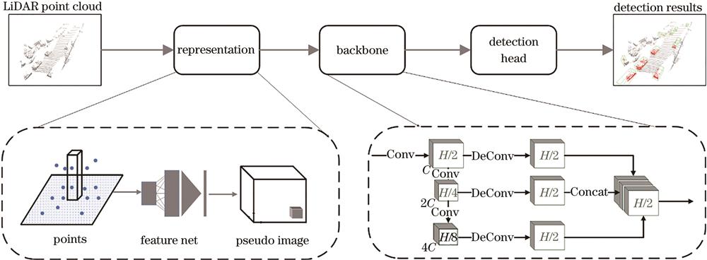
Fig. 1. Flow chart of PointPillars algorithm

Download full size

Fig. 2. Visual effect of original PointPillars detection

Download full size

Fig. 3. Improved feature sampling module

Download full size

Fig. 4. Lidar point cloud removal of ground parts

Download full size

Fig. 5. Point cloud data enhancement. (a) Raw point cloud; (b) mirrored point cloud; (c) tilted point cloud; (d) zoomed point cloud

Download full size

Fig. 6. Comparison of experimental results for hyperparameter selection

Download full size

Fig. 7. Comparison of detection accuracy before and after algorithm improvement

Download full size

Fig. 8. Comparison of detection effects before and after algorithm improvement

Download full size

Model	Depth	Head
M1	（1，3，1）	（2，4，8）
M2	（2，6，2）	（2，4，8）
M3	（2，2，6）	（2，4，8）
M4	（2，6，2）	（2，4，2）
M5	（4，8，4）	（4，8，4）

Table 1. Hyperparameter configuration of Swin-T module

Model	Easy	Moderate	Hard	Average
M1	50.17	40.42	38.7	43.09
M2	94.12	89.55	88.48	90.71
M3	94.23	89.77	88.8	90.93
M4	94.13	89.23	88.15	90.5
M5	94.57	89.65	88.75	90.99

Table 2. Comparison of accuracy rates of different Swin-T hyperparameter configurations

Model	Easy	Moderate	Hard	Average
PointPillars^［6］	90.77	89.61	88.47	89.61
SECOND^［5］	90.76	89.77	88.82	89.78
SECOND-IoU^［5］	89.72	88.73	88.33	88.92
PointRCNN^［21］	90.76	89.58	89.03	89.79
PointRCNN-IoU^［21］	90.70	89.32	88.87	89.63
Part-A2-Free^［22］	90.68	89.00	88.64	89.44
AS-PointPillars^［12］	90.48	88.32	86.51	88.44
AP-PointPillars^［12］	90.68	88.92	86.90	88.83
Proposed model	94.23	89.77	88.8	90.93

Table 3. Comparison of test results

Model	GPU memory /MB	Running speed /s
PointPillars	1267	0.036
Proposed model	1359	0.058

Table 4. Comparison of GPU memory usage and running speed before and after algorithm improvement

Dejiang Chen, Wenjun Yu, Yongbin Gao. Lidar 3D Target Detection Based on Improved PointPillars[J]. Laser & Optoelectronics Progress, 2023, 60(10): 1028012

Download Citation

Set citation alerts for the article

Tools

Set citation alerts for the article

Save the article for my favorites

Paper Information