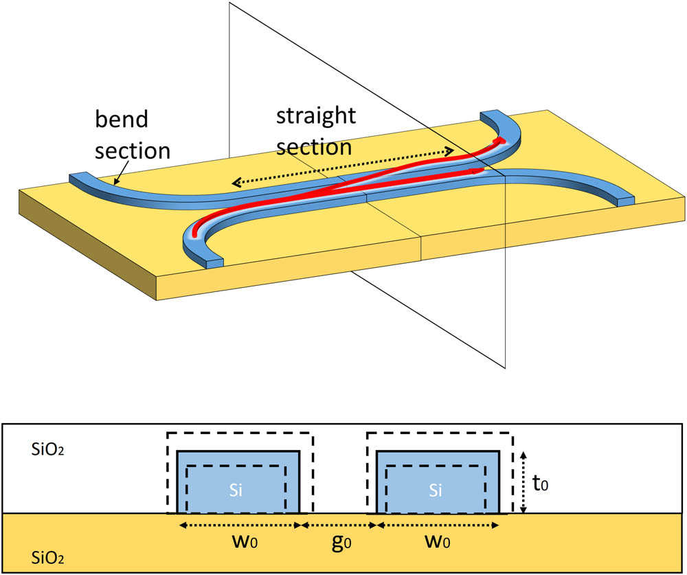
Fig. 1. Upper plot shows the perspective view of a symmetric DC. Red arrows present the flow of light. Part of the light is coupled from bottom waveguide to the above one. Cross section is amplified in the lower plot. The mean width and thickness of the DC are w0 and t0, respectively. The width w and thickness t of the fabricated DC are indicated as dashed boxes. The refractive indexes are nsi=3.44, nSiO2=1.45.

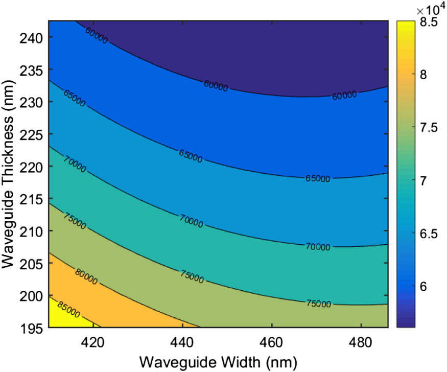
Fig. 2. 2D contour plot of field coupling coefficient versus waveguide width and thickness.

Fig. 3. Flow chart of the proposed technique.

Fig. 4. Top: the red exes (×) represent the interpolation nodes for the normalized independent random variables ξ1 and ξ2 used to build the SC model. Bottom: the blue circles (°) are the corresponding values for the correlated random variables w and t used to compute the coupling coefficients in Fimmwave.

Fig. 5. Sampling points used to perform the MC analysis through direct Fimmwave simulations for the correlated random variables (w,t). The corresponding values for the independent random variables (ξ1,ξ2) are used to evaluate the SC model computed.

Fig. 6. Blue circles (°): coupling coefficient computed via the MC analysis for the 10000 (w,t) samples shown in Fig. 5. Red (×)-markers: corresponding values obtained by evaluating the SC model.

Fig. 7. PDF and CDF of the coupling coefficient for λ=1.55  μm. The blue solid and red dashed line are PDF and CDF obtained by means of the SC model, respectively, while the blue circles and red squares represent the same quantities computed by means of the MC analysis.

Fig. 8. PDF and CDF of the 3 dB-coupling length for λ=1.55  μm. The blue solid and red dashed line are PDF and CDF obtained by means of the SC model, respectively, while the blue circles and red squares represent the same quantities computed by means of the MC analysis.

Table 1. Performance Summary of SC and MC Simulation

Table 2. Computation Time of SC and MC Simulation