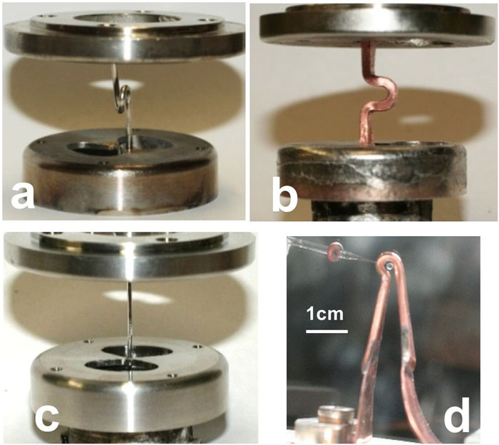
Fig. 1. (a) Spiral, (b) half-turn coil, and (c) rod loads for generating magnetic fields; the anode–cathode gap is 2 cm. (d) Coil load installed with no return-current cage.

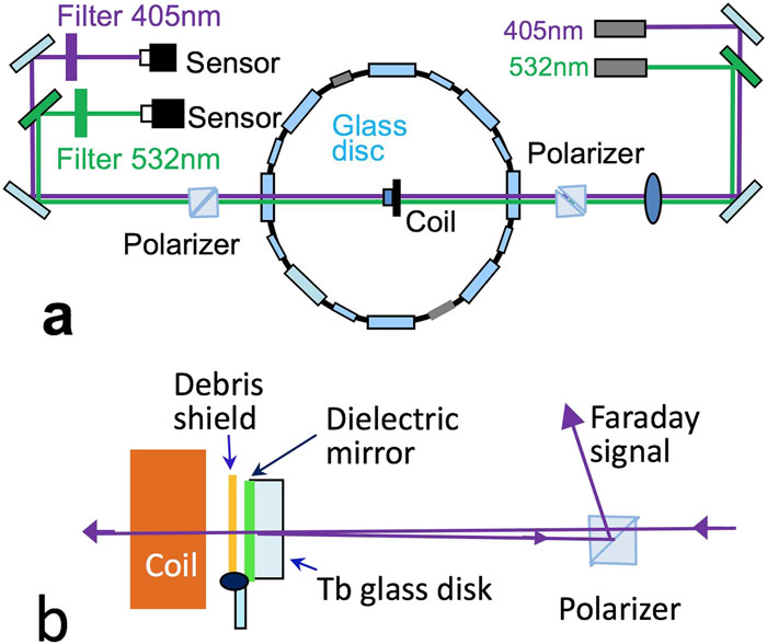
Fig. 2. (a) Two-color CW Faraday-rotation diagnostic. (b) Back-reflected Faraday-rotation diagnostic.

Fig. 3. (a) Current pulse (red) and Faraday-rotation signals at 405 nm (violet) and 532 nm (green). (b) Glass disk near rod load. (c) Current pulse (red) and Faraday signals at 532 nm in half-turn coil. The black line shows the signal from the back-reflected beam and the green line shows the signal from the beam that passed through the coil.

Fig. 4. (a) Faraday target in coil. (b) Current pulse (red line) and magnetic field in 2.5-mm Ta coil (blue line) and on Al rod load with 0.9 mm initial diameter (black).

Fig. 5. (a) Cutoff of Faraday signal in Cu coil without cage as detected with two-color diagnostic. (b) Cutoff in spiral load as detected with back-reflected diagnostic. The photographs show the loads, which correspond to those in Figs. 1(d) and 1(a), respectively.

Fig. 6. (a) and (b) Glass samples near spiral coil. (c) The current and laser beams passed through the coil (blue) and through the glass and coil (green).

Fig. 7. (a) Current pulses (red lines), x-ray pulse from discharge, and transmission in glass plates with thicknesses of 0.2 and 1.4 mm placed near a spiral load. The squares show the coefficient of induced absorption K in the glass. (b) Transmission in 1-mm-thick glass plate protected by a ceramic disc.

Fig. 8. (a) Experimental setup for measuring B-field in tube. (b) Tube in coil. (c) CU tube with slit. (d) Magnetic field in tube center reconstructed from Faraday rotation angle.

Fig. 9. (a) Soak-in time τ calculated by Eq. (2) from Fig. 8(c) for Cu and stainless-steel tubes. (b) τ for Cu tubes with and without slit. (c) and (d) Shadowgraphs of Cu tube (c) before and (d) during shot. Image (e) shows a side view of the cylinder inside the coil.

Fig. 10. (a) Experimental setup for laser–plasma interaction. (b)–(d) Side-on shadowgraphs and interferogram of plasma jets at three wavelengths in one laser shot.

Fig. 11. (a) and (c) End-on schlieren images. (b) and (d) Interferograms. (e) Side-on shadowgraph of plasma disc with tilted probing beam.

Fig. 12. (a) Density and (b) temperature of ablated plasma in 3-MG external magnetic field calculated 4 ns after end of laser pulse.

Fig. 13. (a) Interferogram and (b) shadowgraph of Si target during current and magnetic field in coil load 7 ns after laser pulse. (c) Schematic of laser beam (L) and target (T) near coil load.

Fig. 14. Squares: position of jet tip. Dashed line: MHD simulation.

Fig. 15. (a) Electron density and width of plasma jet reconstructed from interferogram.

Fig. 16. Two-dimensional MHD simulation of electron density of plasma jet 6 ns after laser pulse. The laser pulse irradiating the target comes from the left along the axial magnetic field, and the target is at R = 0.

Fig. 17. (a) Spectrum of 3ω/2 harmonics for Al rod load taken by ICCD with a 3-ns gate. (b) Spectrum for Ni load.

Table 1. Parameters of tubes and the B-field inside.