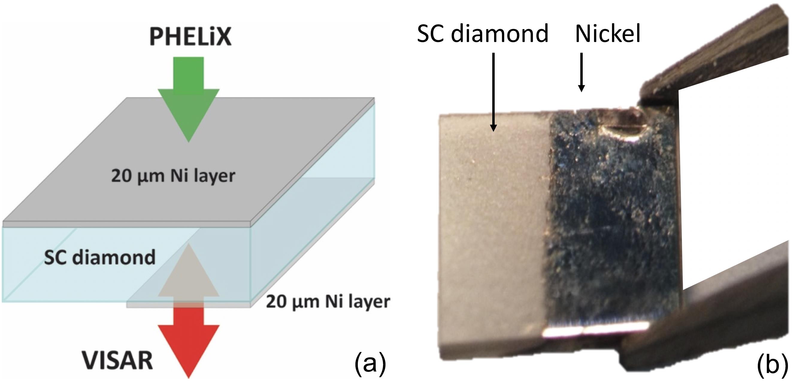
Fig. 1. (a) Scheme of the target used in the experiment and (b) image of Ni layer deposited on target rear side (taken before deposition of the Ni layer on the target front side).

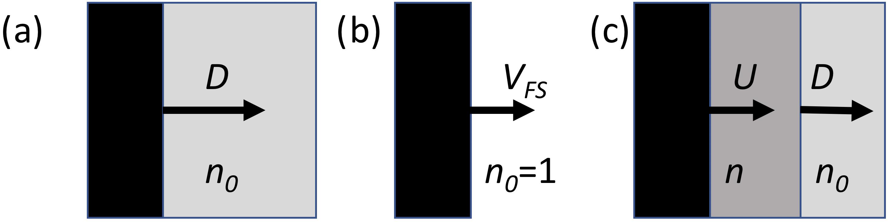
Fig. 2. Reflection of the VISAR probe beam: (a) from a reflecting shock traveling in the material; (b) from a free surface travelling in vacuum; (c) from a reflecting surface embedded in a compressed transparent material.

Fig. 3. VISAR streak camera images from shot 15: (a) VISAR with sensitivity S = 11.3 km/(s·fringe); (b) VISAR with sensitivity S = 4.62 km/(s·fringe). The total time windows are 32.98 ns for VISAR1 and 30.47 ns for VISAR2. Images were recorded on a 16-bit CCD with 1280 × 1024 pixels giving a conversion of ∼30 ps/pixel.

Fig. 4. Time history of the shock velocity in diamond obtained by analyzing the fringe shift of the two VISARs from shot 15 (Figure 3). Here t = 0 is the time of shock breakout at the inner nickel/diamond interface and the shock breakout at diamond rear side takes place 13.48 ns afterwards. The first part of the graph represents the shock velocity in diamond. The second part shows the free surface velocity of diamond after shock breakout at the target rear side.

Fig. 5. (a) Density map of hydrodynamic simulations from MULTI 1D reproducing shot 15. (b) Pressure map of the same shot. (c), (d) Hydrodynamic simulations with the Ni step. Such plots allow the free surface velocity to be estimated for the Ni step and the diamond layer, respectively.

Fig. 6. Result of MULTI 2D simulation. Pressure map (in cgs units) at 14.3 ns within a 300 μm thick target irradiated by a 0.53 μm laser, flat top in space (spot diameter 500 μm) and time (duration 1 ns) with intensity 9 × 10¹³ W/cm².

Fig. 7. Phase diagram of carbon according to Grumbach and Martin^[7] and shock Hugoniot from the SESAME table 7834. The two dashed horizontal red lines show the range of pressures reached in diamond in our shot 15.

Fig. 8. Comparison of phase diagram of carbon from Benedict et al.^[11] and by Grumbach and Martin^[7]: black, the boundaries among different phases according to Ref. [7]; blue, boundaries according to Ref. [11]; green, Hugoniot from SESAME table 7834; red, theoretical Hugoniot from Ref. [11]; thick black, experimental Hugoniot from Eggert et al.^[37].

Fig. 9. Energy gap versus temperature and electron density in the conduction band calculated using the formula from Varshni (constant density, effect of temperature only) and that from Bradley et al. (along the Hugoniot). In this last case, the temperature has been related to compression through SESAME table 7834. For comparison we also show the case in which there is no variation of density and variation of energy gap (i.e., the increase in temperature only affects the Fermi–Dirac distribution of electrons).

Table 1. Obtained experimental results using shock chronometry. We report the thickness of the diamond layer, the laser energy, the shock breakout times from VISAR data, and the corresponding shock velocities. For the first layer, the shock velocity is just an average value obtained by dividing the total 25 μm thickness (plastic ablator + first nickel layer) by the shock breakout time.

Table 2. Comparison of experimental and numerical results for shot 15. Simulations were performed using the SESAME table 7830.

Table 3. Comparison of experimental and numerical results for all shots (note that the laser intensity reported in this table is the intensity used in hydro simulations in order to reproduce experimental data).