Dim small targets detection based on horizontal-vertical multi-scale grayscale difference weighted bilateral filtering

Han-Lu ZHU; Xu-Zhong ZHANG; Xin CHEN; Ting-Liang HU; Peng RAO

doi:10.11972/j.issn.1001-9014.2020.04.016

Abstract

In order to effectively detect weak and small infrared targets under complex background, a single-frame method based on horizontal-vertical multi-scale grayscale difference （HV-MSGD） is proposed to enhance weak targets, and the strong edges of background are suppressed by the difference between the distance and grayscale values. There is discontinuity between the target area and the surrounding area. To strengthen their differences, HV-MSGD combined with bilateral filtering （BF） can increase the intensity of the target while suppressing the background. Candidate targets are further extracted by adaptive local threshold segmentation and global threshold segmentation. In order to further verify the impact on single-frame detection, the above-mentioned single-frame detection algorithm is combined with an improved untraced Kalman particle filter （UPF） to implement trajectory detection. The experimental results show that this method is better than other methods under weak signal-to-noise ratio （SNR）. It can enhance the target while suppressing the background, and the enhancement effect is 6-30 times that of other methods. In the experiments, the input signal-to-noise ratios were 2.78, 1.77, 1.79, 1.13, and 1.16, respectively. After image processing, the background suppression factors （BSFs） are 13.48, 21.33, 11.73, 20.63, and 121.92, and the signal-to-noise ratio gains （GSNRs） are 40.09, 71.37, 27.53, 12.65, and 131, respectively. The probability of detection （Pd） of this method is also superior to other algorithms. When the false alarm rates （FARs） are

5 \times 10^{- 4}

1 \times 10^{- 3}

1 \times 10^{- 3}

1 \times 10^{- 5}

, and

7 \times 10^{- 6}

, the Pd values of the five sets using real sequence images are calculated to be 94.4%, 92.2%, 91.3%, 95.6% and 96.7% respectively.

Keywords

dim target detection distance and pixel difference global threshold segmentation local threshold segmentation multi-scale grayscale difference

Introduction

Prior knowledge of the shape, size, and texture of dim small target is almost non-existent which limits the development of infrared searching and tracking systems [1 - 5] . In general, the background is correlated in both the spatial and temporal domains and primarily occupies low-frequency components in the infrared image, whereas the target is less correlated with background and noise, and mainly occupies high frequency components in the image. When such a target is detected under the space-based platform, the background is generally complex with the small target typically appearing against a background of clouds or water, causing the target to become submerged in clutter and background. In situations such as these, it is difficult to separate the target from the complex background, and the filtering process includes a large amount of edge information. This led to the proposal of algorithms capable of protecting the edges while suppressing the background [6 - 8], such as anisotropy （PM） [9 - 11] and bilateral filter （BF）; [12 - 14] however, these algorithms do not have the ability to separate the background gradient and target gradient. Dim small targets are discontinuous with their neighboring regions in the image and are concentrated in relatively small areas, which can be considered as uniform and dense regions. The discontinuity is essentially based on the average grayscale difference between adjacent pixels. [15] Researchers proposed local measurement methods to establish different regions and surrounding regions in the image, such as the local entropy operator [15 - 21] and local mutation weighted entropy, [22 - 23] which can effectively measure the target area and surrounding area. However, the difference between the measured object and the background grayscale information did not allow the separability of the background gradient and target gradient to be improved.

Based on the above analysis, this study involved the design of a horizontal-vertical multi-scale grayscale difference （HV-MSGD） weighted bilateral filtering （BF） method to detect dim small targets using infrared imaging. The method has the following advantages: （1） the method measures the discontinuity between the target area and background area by comparing the regional standard deviation to determine the size of the window; （2） the HV-MSGD weighted operator is used to realize the expansion of the difference between the target and background area by using the size of the window to achieve target enhancement; （3） background edge information is suppressed in consideration of the difference between the distance and grayscale value of each pixel in the image; （4） the combination of global and local threshold segmentation （GLTS） prevents extremely strong signals such as those of noise and clutter to influence the target itself, which eliminates noise elements and detects the real target signal. In other words, HV-MSGD is combined with BF to improve the separability of the target and background gradient, thereby increasing the energy of the target while suppressing the edge information in the image. Experiments show that this method is superior to other algorithms in terms of its ability to detect weak targets.

1 Single frame detection of dim targets

1.1　Target signal enhancement—HV-MSGD

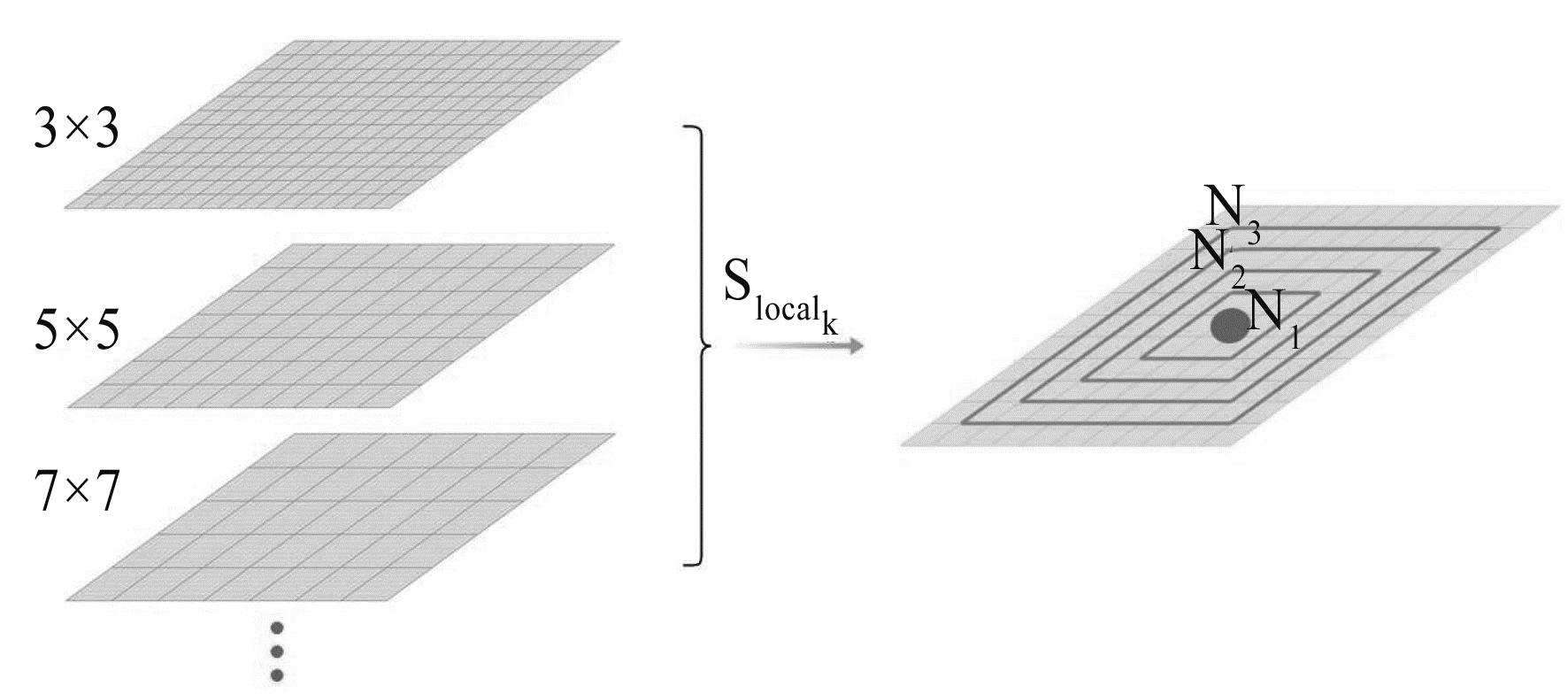
In an infrared image, the grayscale of the target pixels differs greatly from that of the surrounding pixels with a large discontinuity in the luminance. This discontinuity fundamentally determines that the nature of the average grayscale can be obtained from the pixels adjacent to the target. [24] This led researchers to use multi-scale grayscale methods to quantitatively analyze images to distinguish the difference between the target and the surrounding area. [25 - 27] These methods mainly rely on image entropy to obtain multi-scale grayscale difference, the amount of calculation is huge, and the effect on weak targets is not obvious. These attempts encouraged us to develop an improved multi-scale grayscale difference method to enhance the weak signals and to overcome situations in which the thermal intensity measurements of the target are similar to the those of the background.

Small and weak targets are concentrated in a small, uniform and compact area, which has discontinuity with the surroundings. Therefore, this paper designs a method to calculate this discontinuity and achieve enhancement of weak targets. The standard deviation of the image reflects the clutter fluctuations of the images, so the appropriate window size can be selected to obtain the MSGD of the image by comparing the LG-SGD.

The image is traversed from top to bottom and left to right, and the area is divided into neighborhoods surrounding the pixels. As shown in Fig. 1, taking as an example, , and are three differential regions surrounding the central pixel, and the sizes of their windows are , and , respectively. The grayscale average of the th region is expressed as:

v_{N_{k}} = \frac{1}{n_{N_{k}}} \sum_{(m, n) ϵ N_{k}} I (m, n)

Figure 1.

where is the number of differential regions with values k=1,2,3, ..., k, the set represents the differential region, represents the number of pixels in region , and represents the grayscale of pixels in the region . In actual operation, the sizes of windows 3, 5, 7, 9, and 11 are primarily used for calculations and selections. Then the local standard deviation in the kth region is as follows:

S_{l o c a l_{k}} = \frac{1}{n_{N_{k}}} \sqrt[]{\sum_{(m, n) ϵ N_{k}} (I (m, n) - v_{N_{k}})^{2}}

According to Eq. 2, for a heterogeneous region, the local grayscale standard deviation is large when the window is small, whereas the local grayscale standard deviation is small for a homogeneous region in the same window. Figure 2 shows the response of different boundaries at different scales, with the peak response of the horizontal or vertical boundary appearing in a large window. In contrast, a strong peak response occurs at the point target in a small window, indicating that a small-scale window affects the intensity of the point target, but has no effect on the boundary. Thus, selection of a window of the appropriate size can enhance the signal of the target. The size of the window can be determined by comparing the standard deviation within a region:

W_{s i z e} = \underset{W_{s i z e}}{a r g m i n} (S_{l o c a l_{1}}, S_{l o c a l_{2}}, \dots, S_{l o c a l_{k}})

Figure 2.The response of different boundaries at different scales

The determined window size is used to obtain the grayscale value of the predicted point by using the HV-MSGD, and enhancement of the target area is achieved by the difference in response between the horizontal and vertical boundaries. The specific implementation is shown in Fig. 3 . First, the gradient difference of the vertical grayscale is calculated by Eqs. 1-2, after which these two equations are used to calculate the gradient difference of the horizontal grayscale before the results with the enhanced target is obtained. The specific calculation process is as follows:

\begin{array}{l} [\begin{matrix} f_{11} & \dots & f_{n 1} \\ ⋮ & ⋱ & ⋮ \\ f_{1 n} & \dots & f_{n n} \end{matrix}] \overset{V G D}{\Rightarrow} [\begin{matrix} \sum_{i = 1}^{n} (f_{1 i} {- \frac{1}{n} \sum_{i = 1}^{n} f_{1 i})}^{2} & , \dots, & \sum_{i = 1}^{n} (f_{n i} {- \frac{1}{n} \sum_{i = 1}^{n} f_{n i})}^{2} \end{matrix}] \\ = [\begin{matrix} V G D_{11} & , \dots, & V G D_{1 n} \end{matrix}] \overset{H G D}{\Rightarrow} \sum_{i = 1}^{n} (V G D_{1 i} {- \frac{1}{n} \sum_{i = 1}^{n} V G D_{1 i})}^{2} = = H V G D (x, y) \end{array}

Figure 3.calculate the HV-MSGD weighting operator

where is the corresponding value of the region, the horizontal grayscale value is obtained after the vertical gradient difference is calculated, then the final target enhancement value is obtained by calculating the horizontal grayscale gradient difference. In summary, the specific processing of this algorithm is shown in the following module:

Image	Input		BF		TDLMS				PM
Image	$S N R_{i n}$	$σ_{i n}$	BSF	GSNR	BSF		GSNR		BSF	GSNR
Image 1	2.78	30.05	2.15	6.56	8.19		8.5		1.73	3.26
Image 2	1.77	42.87	4.08	13.12	18.72		7.98		1.33	3.12
Image 3	1.79	59.95	1.82	4.33	6.37		4.57		1.77	4.33
Image 4	1.13	36.73	1.38	8.19	11.77		4.92		0.69	1.5
Image 5	1.16	29.26	7.1	20.89	31.46		14.24		2.56	7.12
Image	LCM			NWIE				Our method
Image	BSF		GSNR	BSF		GSNR		BSF		GSNR
Image 1	2.63		7.7	4.55		1.59		13.48		40.99
Image 2	2.63		8.89	4.43		18.94		21.33		71.37
Image 3	1.61		2.98	2.72		16.98		11.73		27.53
Image 4	1.09		1.92	8.46		7.82		20.63		12.65
Image 5	4.41		4.59	21.52		21.32		121.92		131

Table 1. BSF and GSNR of different five images processed by different methods

View all Tables

1.2　Background estimation—BF

Bilateral filtering can smooth the image while estimating the background of the image. The filter employs two weights: the filter coefficient determined by the geometric spatial distance and the filter coefficient determined by the difference in grayscale similarity. In the sampling procedure, which considers the relationship between pixels by using the spatial distance and grayscale similarity difference, the two coefficients are expressed as follows:

c (x, y) = e^{- \frac{(x^{2} + y^{2})}{2 σ_{d}^{2}}}

s (x, y) = e^{- \frac{(f (ξ, η) - f {(x, y))}^{2}}{2 σ_{s}^{2}}}

The weight coefficient is composed of the two:

w_{d s} (x, y) = c (x, y) ∙ s (x, y)

where and are the bandwidth coefficients of the two filter coefficients, is grayscale gray of the region of , then the background estimation can be obtained:

h (x, y) = (\sum_{N \times N} w_{d s} {(x, y))}^{- 1} ∙ \sum_{N \times N} f (x, y) ∙ w_{d s} (x, y)

Subtracting the result of the background estimation from the original image, the background suppression image is obtained as follows:

o u t (x, y) = f (x, y) - h (x, y)

where the is the final background suppression image. It is worth noting that the image needs to be normalized during the calculation process. Then the candidate target is extracted by GLTS.

1.3　Threshold segmentation

The target and its background are discontinuous [15 - 16] . The image is processed by HV-MSGD weighted BF, which enlarges the discontinuity between the target region and the background region. This method successfully enhances the target, and restrains the background clutter and noise effectively. The overall process to detect a dim small target is illustrated in Fig. 4 .

Figure 4.The detection process of the entire dim small target

The threshold segmentation process adopts a method that combines global and local threshold segmentation to determine dim small targets. The global threshold segmentation is an adaptive threshold segmentation for the entire image and is obtained as follows:

T_{G} = t \times σ + m

S e g_{G} = \{\begin{matrix} 1 I m g_{p r o} (i, j) > T_{G} \\ 0 I m g_{p r o} (i, j) \leq T_{G} \end{matrix}

where is the standard deviation of the image, m is the average of the image, and is an odd number greater than 3. Then we can get the image of global threshold segmentation by Eq. 11. is the grayscale value of the image processed by HV-MSGD weighted BF at point . Local threshold segmentation divides the image into regions and calculates the th segmentation threshold value for different regions respectively, using Eq. 12:

T_{L i} = t \times σ_{i} + m_{i}

S e g_{L} = \{\begin{matrix} 1 I m g_{p r o} (i, j) > T_{L i} \\ 0 I m g_{p r o} (i, j) \leq T_{L i} \end{matrix}

where is the standard deviation of the th partition region, =1,2,3, \dots, , and is the average of the th partition region. Then we can get the image of local threshold segmentation by Eq. 13. The algorithm is designed to detect an entire single-frame containing a small target is described in the following module. The two equations use the same threshold .

S e g = S e g_{G} ∙ S e g_{L}

IMAGE	Frame number	Input		BF		TDLMS				PM
IMAGE	Frame number	$\bar{σ_{i n}}$	$\bar{S N R_{i n}}$	$\bar{B S F}$	$\bar{G S N R}$	$\bar{B S F}$		$\bar{G S N R}$		$\bar{B S F}$	$\bar{G S N R}$
Seq 1	75	25.72	2.23	3.13	4.36	1.01		3.58		3.1	2.31
Seq 2	90	8.36	0.56	1.22	5.72	2.42		5.12		1.28	4.56
Seq 3	65	6	1.21	9.3	10.68	2.55		8.24		6.16	7.37
Seq 4	90	32.78	2.09	2.64	9.49	5.71		7.61		1.19	4.01
Seq 5	90	11.53	1.17	1.07	6.77	1.2		4.86		1.95	3.89
Average	-	17.22	1.44	3.12	7.32	2.64		5.82		2.51	4.33
IMAGE	Frame number	LCM			NWIE				Our method
IMAGE	Frame number	$\bar{B S F}$		$\bar{G S N R}$	$\bar{B S F}$		$\bar{G S N R}$		$\bar{B S F}$		$\bar{G S N R}$
Seq 1	75	3.1		1.27	1.98		6.04		5.38		33.97
Seq 2	90	1.01		2.02	2.40		9.42		5.46		15.64
Seq 3	65	4.76		3.13	1.34		13.73		14.71		55.18
Seq 4	90	1.17		7.94	3.17		10.25		23.26		81.8
Seq 5	90	2.94		1.61	1.74		13.1		7.47		47.51
Average	-	2.45		3.27	2.13		10.51		11.26		36.47

Table 2. the average of BSF and GSNR for five sequences

View all Tables

2 Trajectory detection

On the basis of the procedure for single-frame detection described in Sec. 2, further verification of the effect of the proposed method, combined with the improved UPF, is conducted by predicting the target position by the probability data association （PDA） and to finally obtain the motion trajectory. According to the actual moving speed of the target, the frame rate and other factors, setting the range of the suspected position to 10 pixels, to solve the tracking accuracy. For the improved UPF, we detect the single-frame according to Sect. 1, to obtain the positions of suspected target points, and then estimate the suspected target points probabilistically to obtain the predictive value, and according to literature [28] we can get the final target position. For the PDA, we can get the associated probability by following:

β_{i} (k) = \frac{e_{i} (k)}{b (k) + \sum_{j = 1}^{m_{k}} e_{j} (k)} (i = 1,2, \dots, m_{k})

\begin{array}{l} e_{i} (k) = e x p {- \frac{1}{2} [Z (k) - \hat{Z} {(k | k - 1)]}^{T} \\ X^{- 1} (k) [Z (k) - Z (k | k - 1)] \} \end{array}

b (k) = λ {(2 π)}^{\frac{m}{2}} | X (k) |^{\frac{1}{2}} (1 - P_{d} P_{G}) / P_{d}

where represents all valid measurement sets that fall within the target tracking gate at time , represents the number of effective measurement at time , is covariance matrix, is the detection probability with a value of 1, is the threshold probability with a value of 0.97. The steps of the process are shown in Fig. 5 and the specific algorithm is described in Algorithm 3:

Figure 5.Flow chart of trajectory detection

$P_{d}$	Seq 1 $\bar{S N R_{i n}} = 2.23$	Seq2 $\bar{S N R_{i n}} = 0.56$	Seq 3 $\bar{S N R_{i n}} = 1.21$	Seq 4 $\bar{S N R_{i n}} = 2.09$	Seq 5 $\bar{S N R_{i n}} = 1.17$	Average $\bar{S N R_{i n}} = 1.44$
BF	0.9200	0.9470	0.8704	0.9253	0.9525	0.9230
TDLMS	0.7202	0.7427	0.4342	0.4765	0.9334	0.6614
LCM	0.6374	0.8439	0.2871	0.9056	0.6738	0.6696
PM	0.5551	0.7645	0.3061	0.8577	0.6338	0.6234
NWIE	0.8477	0.9167	0.5578	0.8614	0.9507	0.8269
Our method	0.9320	0.9577	0.9349	0.9847	0.9761	0.9571

Table 3. AUC of five sequences in different algorithms

View all Tables

3 Analysis of experimental results

3.1　Experimental environment and images

Figure 6.the results of five images that processed by our method, （a） is the input image, （b） is the 3D view of the input image, （c） is the image processed by HV-MSGD, （d） is a 3D image processed by HV-MSGD, （e） is a threshold segmentation image processed by （c）, （f） is a 3D threshold segmentation image processed by （c）

Figure 7.Background suppression results of different algorithms in different scenarios （a） original image, （b） BF filtering result, （c） TDLMS filtering result in literature 15, （d） PM filtering result, （e） LCM filtering result of in literature 24, （f） NWIE, （g） filtering result of our method

3.2　Evaluation method

The performance of these methods was compared by using three indicators, i.e., the gain of the signal-to-noise ratio （GSNR）, background suppression factor （BSF）, and receiver operating characteristic （ROC） curve for the quantitative evaluation of the background suppression and target detection performance. The indicators are defined as follows:

G S N R = \frac{S N R_{o u t}}{S N R_{i n}}

B S F = \frac{σ_{i n}}{σ_{o u t}}

S N R = \frac{| μ_{t a r g e t} - μ_{b a c k g r o u n d} |}{σ_{n o i s e}}

where and are the local SNR of the target before and after background suppression, and are the standard deviations of the local background area of the target before and after background suppression, and are grayscale peak value of the target and background areas, and is the standard deviation of the local background area.

The evaluation index （Eqs. 18-19） was used to compute BSF and GSNR of the image shown in Fig. 7, and the results are listed in Table 1 . The BSF and GSNR results of the images processed by our method are superior to those obtained by other methods. The SNR values used as input were 2.78, 1.77, 1.79, 1.13 and 1.16, respectively. After image processing, the BSF values were 13.48, 21.33, 11.73, 20.63, and 121.92, and the GSNR values were 40.09, 71.37, 27.53, 12.65, and 131, respectively.

Table Infomation Is Not Enable

The ROC curve describes the mutual constraint relationship between the probability of detection （Pd） and the false alarm rate （FAR）. The value of Pd for different values of FAR can be obtained by changing the detection threshold in Eqs. 10 and 12, where and are the values of Pd and FAR, calculated as follows:

P_{d} = \frac{N_{t a r g e t}}{T_{t a r g e t}}

P_{f} = \frac{N_{p i x e l}}{T_{p i x e l}}

where is the number of detected targets, is the number of actual targets, is the number of pixels of the false target, and is the number of all pixel points in the detection images.

Based on the description of ROC, the ROC values of the five sequences are plotted in Fig. 8, which clearly shows that the values of Pd obtained using our method are more accurate than those obtained with the other algorithms. Five sets of images that formed real sequences were processed using FARs of , , , , and to obtain Pd values of 94.4%, 92.2%, 91.3%, 95.6%, and 96.7%, respectively. In addition, we compared the average values of BSF and GSNR for these five sequences obtained with the different algorithms, and present the results in Table 2 . The five sequences contain 75, 90, 65, 90 and 90 images, respectively. Sequence 1 is on thick cloud background, sequence 2 is on bright cloud background, sequence 3 is on bright edge background, and sequence 4 is on blocky cloud background, and sequence 5 is on bright and thick cloud background. In the experiment, the average SNRs were 2.23, 0.56, 1.21, 2.09, and 1.17, respectively. After using our method for image processing, the average BSFs were 5.38, 5.46, 14.71, 23.26, and 7.47, and the GSNRs were 33.97, 15.64, 55.18, 81.8, and 47.51, respectively. The area under curve （AUC） is defined as the area enclosed by the coordinate axis under the ROC curve. Because the AUC can intuitively characterize the superiority or inferiority of each algorithm, we calculated the AUC of five sequences using different algorithms. These results are provided in Table 3 . Moreover, we further verified the effectiveness of our method by using the trajectory detection algorithm mentioned in Sect. 2 to compute the trajectory. Figures 9-10 show the trajectory image and bias pixels, which are within two pixels. The conclusion that can be made from Figs. 9 - 10 are that the proposed method can achieve high probabilities of detection as well as low false alarm rates for different target movements.

Figure 8.ROC of the five sequences

Table Infomation Is Not EnableTable Infomation Is Not Enable

Figure 9.Track of five sequences

Figure 10.Histograms of detected bias pixels obtained by using our method （a） histograms of horizontal detected bias pixels of five sequences, （b） histograms of vertical detected bias pixels of five sequences

4 Conclusions

This study investigated the problem associated with detecting small targets that are weak infrared emitters. Our efforts mainly focused on increasing the discontinuity between the target region and the background region by using HV-MSGD, which improved the separability of the target from the background. In addition, background edge information was suppressed by BF, and the target was finally extracted by the GLTS algorithm. A comparison of the results with those of other methods on five images showed that our method is superior to other methods in both GSNR and BSF, and the enhancement effect is 6\sim30 times that of the other methods. In addition, comparison of the average and of five sequences that include a total of 410 images also confirmed our method to be 5-12 times more effective than other methods. Counting the probability of detection of the five sequences also indicated our method to be significantly more accurate than other methods, with and the average detection probability of our algorithms of 95.71%. The method proposed in this paper has a good effect on the image with obvious grayscale fluctuation in adjacent regions. For images with small fluctuations, the method of this paper needs further improvement. In future research, we plan to develop a more effective detection algorithm for multi-target complex background and occlusion based on the single-frame detection method proposed in this paper.

References

[1] C Q Gao, D Y Meng, Y Yang. Infrared patch-image model for small target detection in a single image. IEEE Transactions on Image Processing, 22, 4996-5009(2013).

[2] K P Luo. Space-based infrared sensor scheduling with high uncertainly: Issues and challenges. Syst. Eng., 18, 102-113(2015).

[3] F Gao, H Li, T Li. Infrared small target detection in compressive domain. Electron. Lett., 50, 510-512(2014).

[4] C Q Gao, T Q Zhang, Q Li. Small infrared target detection using sparse ring representation. IEEE Aerospace and Electronic Systems Magazine, 27, 21-30(2012).

[5] X Yang, Y P Zhou, D K Zhou. A new infrared small and dim target detection algorithm based on multi-directional composite window. Infrared Phys. Technol., 71, 402-407(2015).

[6] X P Shao, H Fan, G X Lu. An improved infrared dim and small target detection algorithm based on the contrast mechanism of human visual system. Infrared Phys. Technol., 55, 403-408(2012).

[7] P Wang, J W Tian, C Q Gao. Infrared small target detection using directional high pass filters based on LS-SVM. Electron. Lett., 45, 156-158(2009).

[10] Y Li, Y Song, Y F Zhao. An infrared target detection algorithm based on lateral inhibition and singular value decomposition. Infrared Physics & Technology, 85, 238-245(2017).

[11] Z M Chen, M C Tian, Y M Bo. Improved infrared small target detection and tracking method based on new intelligence particle filter. Computational Intelligence, 34, 917-938(2018).

[12] F Zhao, H Z Lu, Z Y Zhang. Complex background suppression based on fusion of morphological Open filter and nucleus similar pixels bilateral filter. Infrared Physics & Technology, 55, 454-461(2012).

[13] Spatial and temporal bilateral filter for infrared small target enhancement. Infrared Physics & Technology, 63, 42-53(2014).

[14] H B Tian, E E Department, H V Amp. Infrared small target detection based on bilateral filter and bhattacharyya distance. Nuclear Electronics & Detection Technology, 34, 1159-1163(2014).

[15] H Deng, Y T Wei, M W Tong. Background suppression of small target image based on fast local reverse entropy operator. IET Computer Vision, 7, 405-413(2013).

[16] H Deng, J G Liu, Z Chen. Infrared small target detection based on modified local entropy and EMD. Chinese Optical Letters, 8, 24-28(2010).

[17] C J Li, Y Wei, Z L Shi. A small target detection algorithm based on multi-scale energy cross. IEEE Int. Conf. Robotics Intell. Syst. Signal Process, 2, 1191-1196(2003).

[18] X Z Bai, Y G Bi. PP（. IEEE Transactions on Geoscience & Remote Sensing, 1-15(2018).

[19] K Shang, X Sun, J W Tian. Infrared small target detection via line-based reconstruction and entropy-induced suppression. Infrared Physics & Technology, 76, 75-81(2016).

[20] Z Chen, S Luo, T Xie. A novel infrared small target detection method based on BEMD and local inverse entropy. Infrared Physics & Technology, 66, 114-124(2014).

[21] Y Mao, M Zheng, W Jia. Analysis of small target detection algorithm based on image gray entropy(2016).

[22] G H Peng, H Chen, Q Wu. Infrared small target detection under complex background. Advanced Materials Research, 346, 615-619(2011).

[23] X J Qu, H Chen, G H Peng. Novel detection method for infrared small targets using weighted information entropy. Journal of Systems Engineering and Electronics, 23, 838-842(2012).

[24] C L Philip, H Li, Y T Wei. A local contrast method for small infrared target detection. IEEE Trans. on Geoscience & Remote Sensing, 52, 574-581(2013).

[25] H Deng, X P Sun, M L Liu. Entropy-based window selection for detecting dim and small infrared targets. Pattern Recognition, 61, 66-77(2017).

[26] H Deng, X P Sun, M L Liu. Infrared small-target detection using multiscale gray difference weighted image entropy. IEEE Transactions on Aerospace & Electronic Systems, 52, 60-72(2016).

[27] G Y Wang. Efficient method for multiscale small target detection from a natural scene. Opt. Eng, 35, 761-768(1996).

[28] X P Huang, Y Wang. Kalman filter principle and application: MATLAB simulation. Publishing House of Electronics Industry(2015).