
Zheng Lei, Zongtao Zhu, Yuanxing Li, Yan Liu, Hui Chen. Numerical Simulation of Characteristics of Laser-Hollow Tungsten Inert Gas Coaxial Composite Welding Arc[J]. Chinese Journal of Lasers, 2021, 48(18): 1802011
- Chinese Journal of Lasers
- Vol. 48, Issue 18, 1802011 (2021)
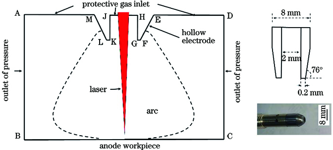
Fig. 1. Schematic diagram of mathematical model of laser coaxial composite arc
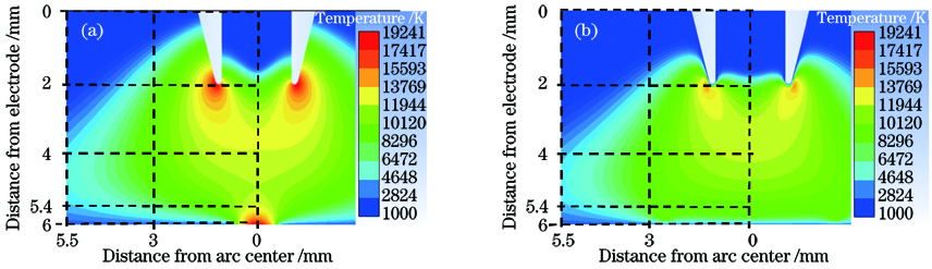
Fig. 2. Cloud diagram of arc temperature distribution. (a) Laser coaxial composite arc; (b) TIG arc
Fig. 3. Comparison of arc temperature
Fig. 4. Cloud diagram of plasma velocity distribution. (a) Laser coaxial composite arc; (b) TIG arc
Fig. 5. Comparison of plasma velocity
Fig. 6. Cloud diagram of arc pressure distribution. (a) Laser coaxial composite arc; (b) TIG arc
Fig. 7. Comparison of arc pressure
Fig. 8. Cloud diagram of arc potential distribution. (a) Laser coaxial composite arc; (b) TIG arc
Fig. 9. Comparison of arc potential
Fig. 10. Cloud diagram of arc magnetic field distribution. (a) Horizontal of composite arc; (b) horizontal of TIG arc; (c) vertical of composite arc; (d) vertical of TIG arc
Fig. 11. Comparison of magnetic field. (a) Horizontal of composite arc; (b) horizontal of TIG arc; (c) vertical of composite arc; (d) vertical of TIG arc
Fig. 12. Arc in experiment. (a) Laser coaxial composite arc; (b) TIG arc
Fig. 13. Welding joint in experiment. (a) Laser coaxial composite arc; (b) TIG arc
|
Table 1. Boundary condition of hollow TIG arc model

Set citation alerts for the article
Please enter your email address
© Copyright 2018-2021 | Chinese Laser Press. All Rights Reserved 沪ICP备15018463号-20