Author Affiliations
1Department of Electrical and Electronic Engineering, Southern University of Science and Technology, Shenzhen 518000, China2Key Laboratory of Intelligent Optical Sensing and Manipulation, Ministry of Education, Nanjing University, Nanjing 210023, Chinashow less
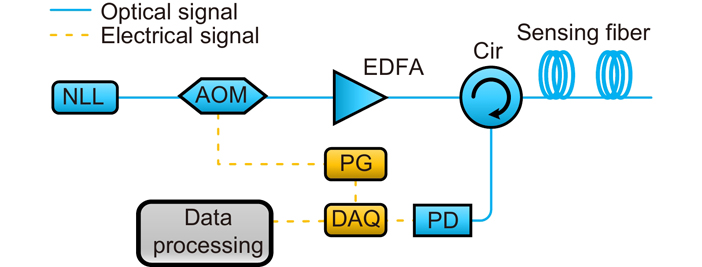
Fig. 1. The setup of DVS-Φ-OTDR system based on direct detection.
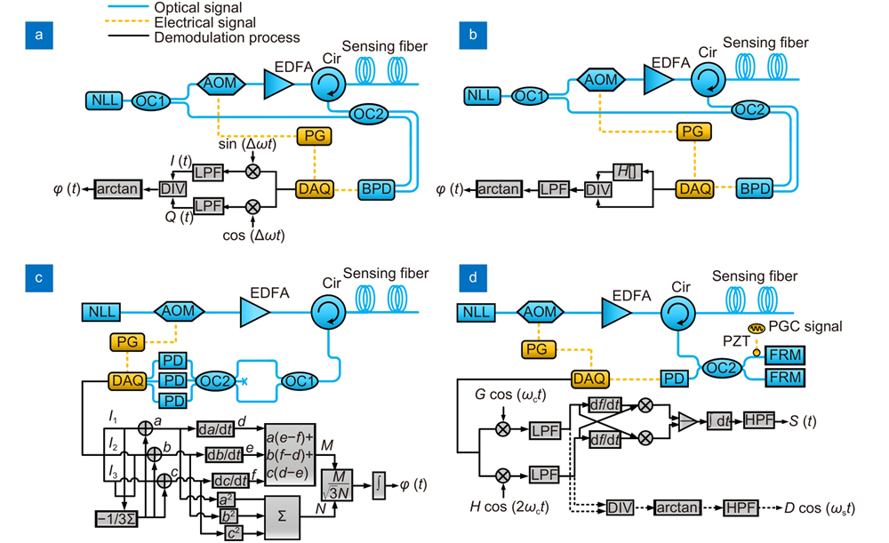
Fig. 2. The setup of DAS-Φ-OTDR system with different demodulation methods.(a) Heterodyne detection + IQ phase demodulation. (b) Heterodyne detection + Hilbert transform phase demodulation. (c) Direct detection + phase demodulation based on a 3×3 coupler. (d) Direct detection + phase demodulation based on PGC.
Fig. 3. Operation principle of Φ-OTDR based VSP monitoring system. (a) Zero-offset VSP. (b) Walk-away VSP.
Fig. 4. (
a) Normalized strain (green curve) recorded during an Mb ~6.2 (USGS) earthquake (Kota Ternate, Indonesia, 2015-03-17 22:12:28 UTC, 1.669°N; 126.522°E, 44 km depth) superimposed with the normalized velocity record (red curve) from the broadband station RAH (80 m from the optical cable). (
b) Zoom-view from (a) showing a good phase correspondence between seismometer velocity record and DAS strain records at a 20s period. (
c) Short record (6 s) of strain phases from a local earthquake trapped in the fault damage zone. Waves inside and outside the fault zone have different apparent velocities. Figures reproduced from ref.
98, under a Creative Commons Attribution 4.0 International License.
Fig. 5. (
a) Stacked DAS beam trace (black) filtered to various bands between 0.02 and 1 Hz compared with amplitude-normalized particle velocity from a broadband seismometer rotated into the mean azimuth of the DAS array (red). (
b) Separation of ocean and seismic waves in the first quadrant of the logarithmic space of the Φ-OTDR signal frequency-wave number domain. Figures reproduced from ref.
101, under a Creative Commons Attribution 4.0 International License.
Fig. 6. Ambient noise based, cross-correlation computed between all Φ-OTDR traces of the cable with respect to one arbitrary trace (at position ~11.5 km) showing several geological features. Figure reproduced from supplementary material of ref.
98 under a Creative Commons Attribution 4.0 International License.
Fig. 7. Experimental site layout. Figure reproduced from ref.
103, under a Creative Commons Attribution 4.0 International License.
Fig. 8. Fiber cable layout and operation principle of 1D-CNN. Figure redrawn after ref.
192.
Fig. 9. An illustration of the railway safety monitoring experiments. Figure reproduced from ref.
108, under the OSA Open Access Publishing Agreement.
Fig. 10. Fiber cable layout alongside railways. Figure redrawn after ref.
113.
Fig. 11. Integration of Φ-OTDR system in the DWDM communication network. Figure reproduced with permission from ref.
116, IEEE.
Fig. 12. Experimental setup for discharge detection with two acoustic transducers attached to the 40 kV joint. (Figure redrawn after ref.
119)
Fig. 13. Fiber deployment inside or outside electrical cable. (Figure redrawn after ref.
120)
Fig. 14. (
a) Fiber coil transducer deployment on the GIS device. (
b) Detected discharge signal of transducer #1, #2 and #3 at pulse repetition rate of 10 kHz. Figure reproduced from ref.
121, under a Creative Commons Attribution 4.0 International License.
Fig. 15. (
a) Φ-OTDR system configuration. (
b) Tree infestation sensing results. (Figure reproduced from ref.
182, under a Creative Commons Attribution 4.0 International License.
Fig. 16. (
a) Cross section of the MCF. The circled fiber cores were selected for bending direction analysis. (
b) Fiber bending direction analysis in the
x-
y-
ε space. The
x-
yplane corresponds to one cross section of the MCF. Figure reproduced from ref.
181, under the OSA Open Access Publishing Agreement.
Fig. 17. (
a) Operation principle of the Φ-OTDR based solar irradiance sensing system. (
b) Temperature difference between the black and reference fiber vs. the applied solar irradiance. Figure reproduced from ref.
183, under a Creative Commons Attribution 4.0 International License.
| Reference | Method | Year | Effect | | ref.15 | Phase-shifted double pulse | 2012 | >20 dB SNR by reducing interference fading | | ref.131 | 0–π binary phase shift + phase-shifted double pulse | 2019 | 46 dB SNR by reducing interference fading | | ref.132 | Multi-frequency nonlinear frequency modulation pulses | 2018 | 45 dB SNR by reducing interference fading | | ref.40 | Three different probe frequencies + a tracking algorithm | 2019 | The fading effect could be suppressed to 1.15% | | ref.133 | Single rectangular probe + a novel spectrum extraction and remixing method | 2019 | 7.1 dB SNR improvement by eliminating interference fading | | ref.134 | Multimode optical fiber + joint independent analysis | 2016 | Eliminate interference fading | | ref.135 | Φ-OTDR system based on uwFBG through an unbalanced 3 × 3 coupler structure | 2017 | 56 dB SNR achievement by reducing interference fading | | ref.136 | Distinguished the false alarm peak by comparison | 2016 | 11.5 dB SNR improvement by discriminating interference fading | | ref.137 | PMF | 2011 | >2 dB SNR achievement by reducing polarization-dependent noise | | ref.138 | Polarization diversity scheme | 2016 | 10.9 dB SNR improvement by reducing polarization-dependent noise | | ref.66 | CDPP +Φ-OTDR system based on uwFBG | 2019 | Eliminate polarization fading | | ref.141 | Wiener filtering technology | 2012 | Reduce phase noise | | ref.16 | Statistics calculating method | 2015 | 6 dB SNR achievement by reducing polarization-dependent noise | | ref.17 | Auxiliary weak reflection points in fiber | 2020 | 60 dB SNR achievement by compensating polarization-dependent noise | | ref.49 | Laser frequency sweep + cross-correlation calculation | 2015 | Suppress the influence of LSFD | | ref.51 | A twice differential method | 2019 | The signal fluctuation induced by LSFD is decreased by more than 13 dB. | | ref.52 | An auxiliary MZI interferometer | 2019 | The low frequency noise is reduced by 10 dB | | ref.71 | 2D-ED | 2013 | 8.4 dB SNR by processing various noises together | | ref.142 | A new positioning method based on power spectrum analysis | 2014 | 19.4 dB SNR by processing various noises together | | ref.72 | 2D-ABLF | 2017 | >14 dB SNR improvement by processing various noises together | | ref.143 | ATMF | 2017 | >10 dB SNR achievement by processing various noises together | | ref.144 | Curvelet denoising | 2017 | 8 dB SNR achievement by processing various noises together | | ref.70 | EMD | 2017 | 2.74 dB SNR improvement by processing various noises together | | ref.145 | Multi-scale matched filtering | 2019 | 6 dB SNR improvement by processing various noises together | | ref.146 | A signal processing method based on CS | 2018 | 34.39 dB SNR by processing various noises together |
|
Table 0. Research progress on improving the SNR in Ф-OTDR systems
| Reference | Method | Year | Sensing distance | | ref.122 | EDFA | 2003 | 25 km | | ref.123 | First-order bidirectional Raman amplification | 2009 | 62 km@100 m SR | | ref.124 | Second-order Raman amplification | 2014 | 125 km@10 m SR | | ref.57 | First-order bidirectional Raman amplification + heterodyne detection | 2014 | 131.5km@8 m SR | | ref.54 | Brillouin amplification + heterodyne detection | 2014 | 124 km@10 m SR | | ref.125 | First-order Raman amplification + second-order Raman amplification + Brillouin amplification | 2014 | 175 km@25 m SR | | ref.126 | B-EDFA | 2016 | 123 km@8 m SR | | ref.127 | RP-EDFA | 2017 | 75 km | | ref.128 | Non-balanced optical repeaters | 2018 | 150 km@20 m SR | | ref.129 | Long pulse + balanced amplified detector + heterodyne detection | 2015 | 60 km@6.8 m SR | | ref.130 | Cascaded AOMs + optimizing system components | 2019 | 94.8 km@10 m SR |
|
Table 0. Research progress on improving sensing distance in Ф-OTDR systems.
| Reference | Feature extraction method | Classification methods | Year | Feature extraction domain | Types of intrusion events | | ref.164 | Level crossing rate | threshold-based decision tree | 2014 | Time-domain | Climbing up the wall + kicking at the wall + watering on the fiber | | ref.165 | SSA | BP ANN | 2014 | Time-domain | Sound interferences + hand perturbation | | ref.166 | Average and variance of the correlation coefficients | threshold-based decision tree | 2017 | Time-domain | Jogging + digging | | ref.104 | SAK | threshold-based decision tree | 2018 | Time-domain | Pencil-break + digging | | ref.142 | Total energy of each sampling point | threshold-based decision tree | 2014 | Frequency-domain | Knocking on the fence with a steel spanner | | ref.167 | Energy information entropy | threshold-based decision tree | 2015 | Frequency-domain | Raindrop + construction machine + train + car | | ref.74 | The total energy + the ratio of the low-band energy to the total energy + the ratio of the peak amplitude to the average value of the spectrum | SVM | 2015 | Frequency-domain | A stable state + walking on the lawn while the fence is exposed to the win + shaking the fence + walking on the lawn + vibration exciter | | ref.73 | The sum of the normalized coefficients of the 10 frequency bands | SVM | 2016 | Frequency-domain | Train tracking | | ref.68 | WT | — | 2012 | Time-frequency domain | PZT vibration | | ref.168 | WD | threshold-based decision tree | 2013 | time-frequency domain | Personal intrusion + hand clapping interferences | | ref.169 | WPD | — | 2014 | Time-frequency domain | PZT vibration | | ref.102 | STFT | GMM | 2016 | Time-frequency domain | Big excavator + small excavator + pneumatic hammer + plate compactor | | ref.69 | HHT | — | 2014 | Time-frequency domain | PZT vibration | | ref.171 | MFCC | CNN | 2017 | time-frequency domain | Human digging + pile driver ramming + air pick hitting + excavator scrapping + environmental noise | | ref.113 | Normalized sliding variance | Threshold-based decision tree | 2014 | Time-space domain | Train tracking | | ref.172 | Morphological features | RVM | 2015 | Time-space domain | Walking + digging + vehicle passing | | ref.173 | Level crossing rate + power spectrum analysis | SVM | 2017 | time-domain + frequency-domain | Taping + striking + shaking + crushing | | ref.174 | Time-frequency entropy + center-of-gravity frequency | PNN | 2018 | Time-domain features + time-frequency domain features | A stable state + tapping + climbing |
|
Table 0. Research progress on event discrimination in Ф-OTDR systems.
| Reference | Method | Year | High frequency response | | ref.147 | MZI | 2013 | 3 MHz in 1064 m | | ref.148 | MZI + TDM | 2013 | 6.3 MHz in 1150 m | | ref.149 | MZI + WDM | 2016 | 50 MHz in 2.5 km | | ref.44 | A pulse pair with a frequency difference | 2014 | 2 times improvement | | ref.150 | TSMF | 2015 | 30 kHz in 3024 m | | ref.42 | A hybrid single-end-access MZI | 2017 | 1.2 MHz in 6.35 km | | ref.43 | DFI | 2018 | 1 MHz in 2.16 km | | ref.151 | FLI | 2020 | 300 kHz in 4 km | | ref.152 | Sagnac interferometer + WDM | 2020 | 2.5 MHz in 4 km | | ref.47 | Double-pulse heterodyne detection | 2018 | 20 kHz in 10 km | | ref.153 | OFDM + a weak reflector array Φ-OTDR | 2020 | 25 kHz in 51 km | | ref.154 | ARS+NLFM | 2019 | 20 kHz in 50 km |
|
Table 0. Research progress on improving frequency response range in Ф-OTDR systems.
| Reference | Method | Year | Spatial resolution | | ref.6 | Heterodyne detection + moving average + moving difference | 2010 | 5 m | | ref.71 | 2D-ED | 2013 | 3 m | | ref.155 | HOC | 2019 | 5 m | | ref.27 | Two separate FBGs + MZI | 2017 | 50 cm | | ref.156 | Two Michelson interferometers + PGC algorithm | 2018 | 0.8 m | | ref.157 | Pulse compression | 2017 | 30 cm | | ref.158 | FSP | 2018 | 0.95 m | | ref.159 | Chirped pulses | 2019 | 10 times improvement |
|
Table 0. Research progress on improving spatial resolution in Ф-OTDR systems.