
Xiongbin Wang, Qiushi Wang, Yulong Chen, Jiagen Li, Ruikun Pan, Xing Cheng, Kar Wei Ng, Xi Zhu, Tingchao He, Jiaji Cheng, Zikang Tang, Rui Chen. Metal-to-ligand charge transfer chirality-based sensing of mercury ions[J]. Photonics Research, 2021, 9(2): 213
- Photonics Research
- Vol. 9, Issue 2, 213 (2021)
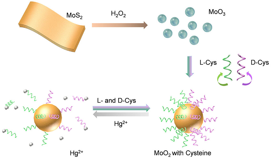
Fig. 1. Illustration of the synthesis process of chiral Cys - MoO 2 Hg 2 +
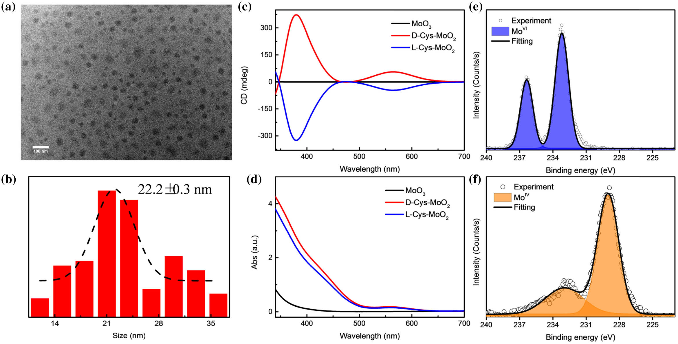
Fig. 2. (a) TEM image of D - Cys - MoO 2 MoO 3 L - Cys - MoO 2 D - Cys - MoO 2 MoO 3 D - Cys - MoO 2
Fig. 3. Chiroptical sensing of Hg 2 + Cys - MoO 2 Hg 2 + D - Cys - MoO 2 L - Cys - MoO 2 Hg 2 + g g Hg 2 +
Fig. 4. (a) TGA curves of L - Cys - MoO 2 L - Cys - MoO 2 L - Cys - MoO 2 Hg 2 +
Fig. 5. TD-DFT simulation for different amounts of D-Cys capped Mo 4 O 8 Mo 4 O 8
Fig. 6. Selectivity of D - Cys - MoO 2 Hg 2 + D - Cys - MoO 2 Zn 2 + Cd 2 + Pb 2 + Ag + Cu 2 + Hg 2 +
|
Table 1. Comparison of the Proposed Probe with Previously Reported a
|
Table 2. Summary of Calculated Mass Loss and Ligand Density for

Set citation alerts for the article
Please enter your email address
© Copyright 2018-2021 | Chinese Laser Press. All Rights Reserved 沪ICP备15018463号-20