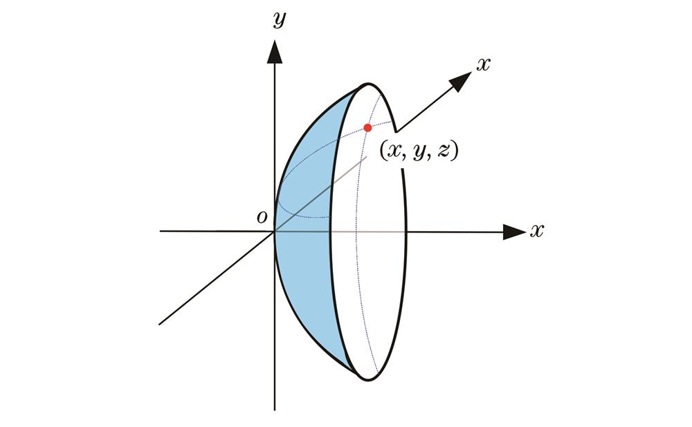
Fig. 1. Description of optical surface based on cartesian coordinate system

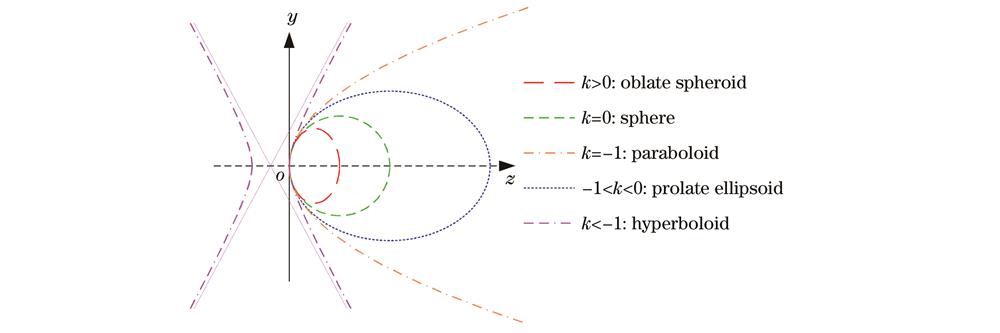
Fig. 2. Profiles of different surface types in yoz plane corresponding to different values of k

Fig. 3. Off-axis conic base surface defined with off-axis angle^[20]

Fig. 4. Schematic diagram of ASAS

Fig. 5. Ultra-thin reflective imaging system^[16]. (a) Optical layout of initial system using even aspheric surface; (b) optical layout of system using ASAS; (c) MTF curves of system using ASAS

Fig. 6. Catadioptric ultra-wide-angle imaging system^[73]. (a) Optical layout of system; (b) MTF curves of system using even aspheric surface; (c) MTF curves of system using ASAS; (d) MTF curves of system after fitting ASAS to even aspheric surface

Fig. 7. Profile of APS in yoz plane

Fig. 8. Ultra-short throw ratio projection objective using APS^[18]. (a) Layout of system; (b) distortion grid of system; (c) MTF curves of system

Fig. 9. Schematic diagram of SSPS^[22]

Fig. 10. Off-axis system with two mirrors and three reflections^[22]. (a) Optical layout of system; (b) design result using traditional xy polynomial surface; (c) design result using SSPS; (d) RMS wavefront error of system using traditional xy polynomial surface; (e) RMS wavefront error of system using SSPS; (f) MTF curves of system using SSPS; (g) distorted grids of system using SSPS

Fig. 11. Off-axis system with three mirrors and four reflections^[22]. (a) Optical layout of system; (b) design result using traditional xy polynomial surface; (c) design result using SSPS; (d) RMS wavefront error of system using traditional xy polynomial surface; (e) RMS wavefront error of system using SSPS

Fig. 12. Description of first-order data of system using freeform surface^[76]. (a) Optical layout of freeform prism; (b) optical layout of system using best-fitting double-curvature biconic surface; (c) Gaussian curvature distribution of best-fitting conic surface of S₃; (d) Gaussian curvature distribution of best-fitting double-curvature biconic surface of S₃

Fig. 13. Fitting error diagram of xy polynomial surface of double-curvature biconic surface converted into xy polynomial surface by different methods^[76]. (a) Least squares method; (b) singular value decomposition method; (c) xy polynomial surface of double-curvature biconic surface is directly converted into x-axy polynomial surface; (d) converted x-axy polynomialsurface is further optimized into xy polynomial surface

Fig. 14. Schematic diagrams of Alvarez system. (a)(d) System is equivalent to negative lens and diverges beam; (b)(e) initial statement of system can be designed as parallel glass plate state or with initial optical power; (c)(f) system is equivalent to positive lens and converges beam

Fig. 15. Optimized Alvarez system. (a) Theoretical optical power P is -10 m^-1; (b) theoretical optical power P is -4 m^-1;(c) theoretical optical power P is 2 m^-1

Fig. 16. Optical power and astigmatism distributions of single lens in optimized Alvarez system. (a) Distribution of optical power; (b) distribution of astigmatism

Fig. 17. Off-axis conic surface^[63]. (a) Off-axis ellipsoid; (b) off-axis hyperboloid

Fig. 18. Optical properties of conic mirrors^[19]

Fig. 19. Ideal imaging off-axis three-mirror system using focus transfer^[19]. (a) Paraboloid-ellipsoid-ellipsoid; (b) paraboloid-hyperboloid-ellipsoid

Fig. 20. Design process of compact off-axis three-mirror system^[19]. (a) Optical layout of initial system using CBS; (b) RMS spot diagram of initial system; (c) optical layout of design using CBR; (d) RMS wavefront error of system using CBR; (e) optical layout of design result using CBN; (f) RMS wavefront error of system using CBN; (g) RMS wavefront error of system after CBNs are converted to traditional xy polynomial surfaces

Fig. 21. Process of integrating two surfaces into single surface^[21]. (a) Coordinates and the normals of sampling points from two original surfaces; (b) local coordinate system of base sphere and freeform surface; (c) freeform surface is obtained by fitting based on the normal of discrete points and residual

Fig. 22. NURBS surface fitted with Peaks surface based on MBA algorithm^[15]. (a) Peaks surface to be fitted; (b) result of 3rd fitting; (c) result of 4th fitting; (d) result of 5th fitting

Fig. 23. Schematic diagram of ray tracing process^[15]

Table 1. NURBS inversion algorithm's efficiency^[15]