
Fengchao Ni, Haigang Liu, Yuanlin Zheng, Xianfeng Chen. Nonlinear harmonic wave manipulation in nonlinear scattering medium via scattering-matrix method[J]. Advanced Photonics, 2023, 5(4): 046010
- Advanced Photonics
- Vol. 5, Issue 4, 046010 (2023)
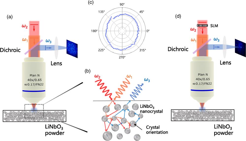
Fig. 1. Schematic of controlling nonlinear light in scattering medium via the scattering-matrix method. (a) Generation of nonlinear speckle pattern without shaping the wavefront of the input fields. (b) Nonlinear signals generation and scattering process in LN powder. (c) Intensity of nonlinear signal for a variable polarization of input field
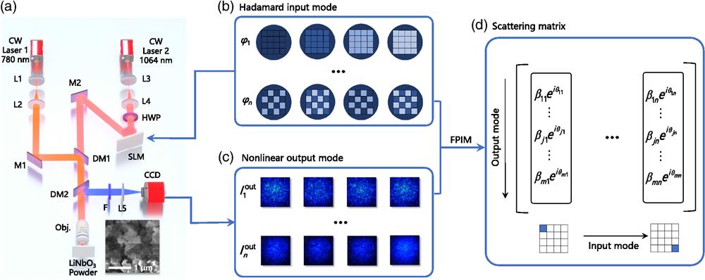
Fig. 2. The SM measurement process. (a) Experimental setup. L1 to L5, lenses,
Fig. 3. Reconfigurable focusing of nonlinear signals via wavefront-shaping method based on SM. (a) Measured SM that connects the input modes (horizontal axis) and output nonlinear modes (vertical axis). Hue and brightness represent phase and amplitude, respectively. (b) Calculated phase patterns for focusing nonlinear signals on different positions of the ROI with superpixel coordinates (3, 5) (red); (9, 9) (blue); (6, 3), and (6, 7) (green, double spots). (c) Focal spots located at different subregions of the ROI with the corresponding optimized phase patterns. (d) Intensity cross section of the nonlinear focal spots located on different subregions of the ROI (red, green, and blue curves).
Fig. 4. Statistical properties of the SM: distribution of the (a), (b) real and imaginary parts of the measured SM and (c) the normalized singular value of the SM. The blue dashed line represents the singular value distribution from the quarter-circle law. Inset: normalized singular value of the matrix after removing the neighboring element. (d) Normalized amplitude profile of the focusing operator
Fig. 5. Nonlinear focusing along predefined trajectories. (a) Predefined scan trajectory in the shape of the letter “S” of the nonlinear focus. The scanning direction is marked by the arrow. (b) Nonlinear focus of each position in the scan path at different times. (c) Actual trajectory of the nonlinear focus in the shape of the letter “S.” (d) Predefined scan trajectories in the shape of the letters “J,” “T,” and “U.” (e) Actual trajectory of the nonlinear focus in the shape of the letters “J,” “T,” and “U.”

Set citation alerts for the article
Please enter your email address
© Copyright 2018-2021 | Chinese Laser Press. All Rights Reserved 沪ICP备15018463号-20