
Yan-Jun Gu, Sergei V. Bulanov. Magnetic field annihilation and charged particle acceleration in ultra-relativistic laser plasmas[J]. High Power Laser Science and Engineering, 2021, 9(1): 010000e2
- High Power Laser Science and Engineering
- Vol. 9, Issue 1, 010000e2 (2021)
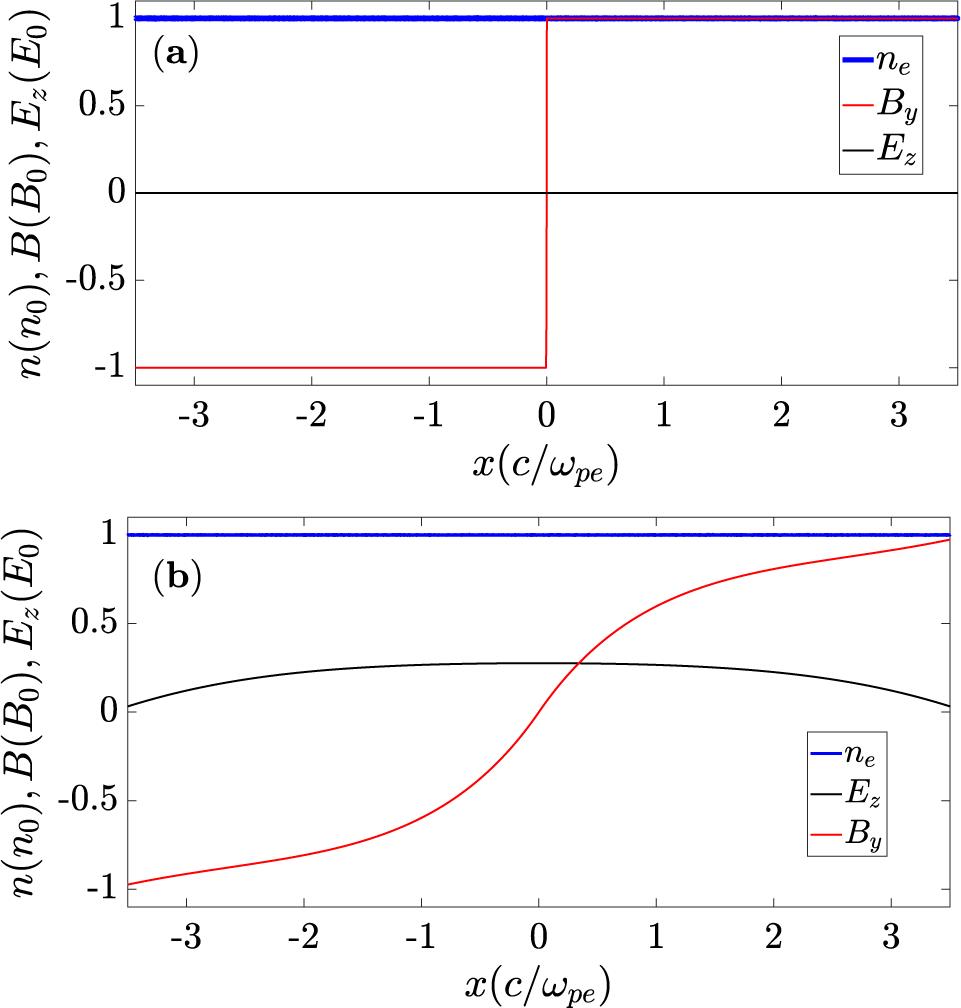
Fig. 1. (a) The initial condition of 1D model. (b) Magnetic field annihilation and electric field growing.
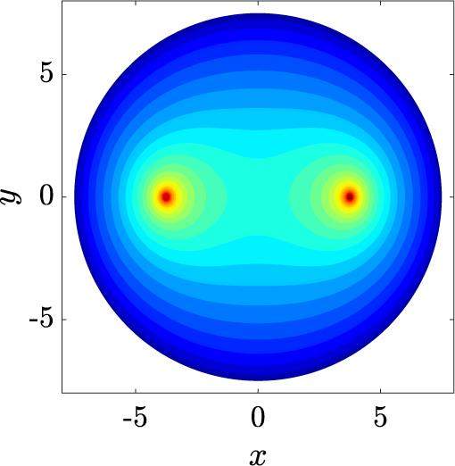
Fig. 2. Contours of equal value of the electric field in the xy plane at  .
.
. Fig. 3. The numerical demonstration of static magnetic field driven by energetic electron beam. (a) The electron density distribution with the plasma channel formation. (b) The blue and red curves represent the longitudinal electric field and the electron density profile on the laser axis ( ). (c) The average energy distribution of the electrons. (d) The
 z component of the azimuthal magnetic field induced by the energetic electron beam.
). (c) The average energy distribution of the electrons. (d) The Fig. 4. (a) The transverse expansion of the magnetic dipole along a density downramp region. The distributions of  at different snapshots are combined here. (b) The profiles of
  along different
  -coordinates.
at different snapshots are combined here. (b) The profiles of along different -coordinates. Fig. 5. (a) The energy density distribution ( ) of electrons. The round circles represent the azimuthal magnetic fields. The projections of
  components in (b) the uniform density region and (c) the density downramp region.
) of electrons. The round circles represent the azimuthal magnetic fields. The projections of components in (b) the uniform density region and (c) the density downramp region. Fig. 6. (a) and (b) are contours of the constant vector potentials around the  -point based on theoretical model. (a) refers to the initial stage when the opposite magnetic fields just begin to vanish. (b) refers to the moment when the current sheet in MR has formed and bifurcated. (c) and (d) are the corresponding distributions demonstrated by numerical simulations.
-point based on theoretical model. (a) refers to the initial stage when the opposite magnetic fields just begin to vanish. (b) refers to the moment when the current sheet in MR has formed and bifurcated. (c) and (d) are the corresponding distributions demonstrated by numerical simulations. Fig. 7. (a) The magnetic field  distributions in the simulation when MR is occurring. (b) The surface represents the distribution of longitudinal electric field (
 ). The curves are the profiles of all the components in Ampere-Maxwell law (
Equation (57) ).
distributions in the simulation when MR is occurring. (b) The surface represents the distribution of longitudinal electric field (). The curves are the profiles of all the components in Ampere-Maxwell law (Fig. 8. The energy distributions of the electrons inside current sheet before and after magnetic field reconnection.
Fig. 9. (a) Schematic of the theoretical model in the vicinity of  -point. (b) The analytical solutions of particles motion with the expressions in
 Equations (96) and (97) . (c) and (d) are the trajectories of charged particles given by the solutions of Equations (98) and (99) for the initial conditions of  ,
,  and
and  . (e) and (f) show the typical accelerated particle trajectories obtained in the kinetic simulations.
-point. (b) The analytical solutions of particles motion with the expressions in , and . (e) and (f) show the typical accelerated particle trajectories obtained in the kinetic simulations. Fig. 10. (a) The intensity distribution of  mode laser on the focused plane and (b) the corresponding profile. (c) The electron density distribution and (d) the
  distribution obtained from numerical simulations in the interaction of
  mode laser with plasma.
mode laser on the focused plane and (b) the corresponding profile. (c) The electron density distribution and (d) the distribution obtained from numerical simulations in the interaction of mode laser with plasma. Fig. 11. (a) The evolution of incident laser intensity before and after interacting with the solid cone target. A loop structure (donut shape) is formed. (b) The electron density distribution driven by the donut shape field. The rear plane corresponds to the density distribution slice of  . The left plane is the projection of the slice of
  . The bottom plane is the projection of magnetic field
  distribution, which shows the magnetic dipoles are formed.
. The left plane is the projection of the slice of . The bottom plane is the projection of magnetic field distribution, which shows the magnetic dipoles are formed. 
Set citation alerts for the article
Please enter your email address
© Copyright 2018-2021 | Chinese Laser Press. All Rights Reserved 沪ICP备15018463号-20