• High Power Laser Science and Engineering
  • Vol. 9, Issue 1, 010000e2 (2021)
Yan-Jun Gu1、2、* and Sergei V. Bulanov1、3
Author Affiliations
  • 1Institute of Physics of the ASCR, ELI-Beamlines, Na Slovance 2, 18221 Prague, Czech Republic
  • 2Institute of Laser Engineering, Osaka University, Osaka565-0871, Japan
  • 3Kansai Photon Research Institute, National Institutes for Quantum and Radiological Science and Technology, 8-1-7 Kizugawa-shi, Kyoto 619-0215, Japan
  • show less
    DOI: 10.1017/hpl.2020.45 Cite this Article Set citation alerts
    Yan-Jun Gu, Sergei V. Bulanov. Magnetic field annihilation and charged particle acceleration in ultra-relativistic laser plasmas[J]. High Power Laser Science and Engineering, 2021, 9(1): 010000e2 Copy Citation Text show less

    Abstract

    Magnetic reconnection driven by laser plasma interactions attracts great interests in the recent decades. Motivated by the rapid development of the laser technology, the ultra strong magnetic field generated by the laser-plasma accelerated electrons provides unique environment to investigate the relativistic magnetic field annihilation and reconnection. It opens a new way for understanding relativistic regimes of fast magnetic field dissipation particularly in space plasmas, where the large scale magnetic field energy is converted to the energy of the nonthermal charged particles. Here we review the recent results in relativistic magnetic reconnection based on the laser and collisionless plasma interactions. The basic mechanism and the theoretical model are discussed. Several proposed experimental setups for relativistic reconnection research are presented.

    1 Introduction

    Magnetic reconnection (MR) rapidly converts the magnetic field energy to the kinetic and thermal energies of the charged particles in plasmas with the topological variations[14]. It is one of the fundamental phenomena in astrophysics and is considered to participate in various processes such as coronal mass ejections[5,6], solar flares[79], closure of the planetary magnetosphere[1012], $\gamma$-ray bursts[1316] and pulsar winds[1719]. In the solar-terrestrial environment where there are full of space plasmas, the study of MR is critical and essential for understanding and modelling the corresponding physical processes.

    MR also plays important roles in laboratory plasmas on fusion instabilities[4,2023] and the weakly ionized plasmas[24]. Early experiments on linear device with highly reproducible plasma presented clear maps of the magnetic fields with movable probe[25]. In the toroidal fusion devices such as Tokamaks, the plasmas tend to relax to a quasi-stationary state via the global magnetic self-organization based on MR process. Based on the features of magnetic field in the toroidal plasmas, the magnetically driven reconnection experiments are performed on the special devices such as magnetic reconnection experiment (MRX)[26,27] and versatile toroidal facility (VTF)[28]. The plasma density on such devices is relatively low being approximately equal to ${\sim}10^{12}\!-\!10^{14}\,\mathrm{cm}^{-3}$ with the corresponding magnetic field strength about kG. Therefore the magnetically driven reconnection occurs in low $\beta$ plasmas where magnetic pressure dominates over thermal pressure. The experiments preformed with MRX and VTF include the study of two-fluid effects on MR with different collisionality[29] and the measurements of spontaneous MR in which energetic ion outflows and rapid electron temperature rise are detected[30]. In addition to the experiments, kinetic theories and simulations also become important tools for MR in laboratory plasmas. Spontaneous magnetic reconnection mechanisms in plasma with tearing-mode instability have been studied[31]. MR in collisionless plasmas has been discussed in detail via particle simulations[3234]. In a weakly ionized plasma, the ampipolar diffusion changes the time and space scale of MR, which makes reconnection faster compared to the case without ion-neutral drift[24].

    The motivations of the studies in MR are mainly inspired by the explanations of the charged particle acceleration mechanisms in space plasmas[3537]. Recent theoretical works discussed about the particle acceleration during the X-point collapse[38,39]. Based on the recent astrophysical observations of 100 MeV gamma flares from the synchrotron radiation of the Crab Nebula detected by Agileand Fermi-LAT[40,41], the high energy photons refer that the accelerated charged particles in the nebula have the energies with a magnitude of PeV. The temporal evolution of the $\gamma$-ray shows that a strong non-stationary electric field accelerates the corresponding emitting electrons. Theoretical and numerical analyses propose that the electron acceleration via the relativistic MR is the potential mechanism explaining this phenomenon[4245]. It arouses an interesting challenge how we can prove such hypothesis by modelling the astrophysical processes under the conditions of terrestrial laboratories.

    The presence of high power laser facilities provides an unique way to investigate MR via laser-plasma interactions. Great progress has been achieved since the invention of the chirped pulse amplification techniques[46]. The state-of-the-art laser intensities exceed ${10}^{22}\ \mathrm{W}/{\mathrm{cm}}^2$[47,48] and the forthcoming facilities are designed to reach more than ${10}^{23}\ \mathrm{W}/{\mathrm{cm}}^2$ with the 10 PW class power[49]. The interactions between ultra-intense laser pulse and plasma generate suprathermal electrons and strong magnetic fields in a short temporal and limited spatial scale. Such properties make the laser-plasma interactions attract more and more attention in recent decades in the MR community. In the pioneering experiments presented on Vulcan laser[50], two nano-second laser pulses with moderate intensities (${\sim}{10}^{15}\ \mathrm{W}/{\mathrm{cm}}^2$) have been used to irradiate on high Z (Au or Al) solid thin foils. According to the Biermann battery effect[51], magnetic fields with the magnitude of mega-Gauss were induced and the plasma jets with high temperature electrons were detected. Four nano-second pulses on OMEGA facility were employed to ablate a plastic (CH) foil[52]. The time-resolved proton deflection technique presented the evolution of the magnetic field in the reconnection process. The experiment performed on SG II facility forced magnetic field lines to reconnect by the collisions of two plasma bubbles[53]. An arc shape X-ray image was obtained and can be used to model the loop-top X-ray source observed in solar flares. In the more recent experiment on SG II, the effects of the external guide magnetic field on the nonthermal electron acceleration were discussed[54]. For the theory of the external guide magnetic field on the nonthermal electron acceleration see Refs. [55,56]. With higher laser intensities, the formation of plasmoids and fan-like ejections with MeV energy was obtained[57]. On the Gekko XII HIPER laser system, the electron scale reconnection was presented in which an external magnetic field was applied in the direction perpendicular to the plasma propagation[58]. In addition to the mentioned representative experiments, there are also a number of theoretical and numerical works focused on MR under the context of laser-plasma interactions. The collisions of magnetized laser-produced plasma bubbles were modeled by magnetohydrodynamics (MHD) simulations[59]. The electrons energization before and during the laser-driven magnetic reconnection was presented by kinetic simulations under the conditions of SG II laser facility[60,61].

    With the increase of laser power, the laser-plasma interactions transit to collisionless relativistic and even ultra-relativistic regime in which high intensity electromagnetic waves, relativistic energetic charged particles are generated[62]. It makes a favourable condition to investigate the relativistic astrophysics processes mentioned above[6365]. The MR in relativistic laser plasmas has been foreseen by Askar’yan et al. who conjectured that the interactions of magnetic field and electron beams under relativistic laser-plasma conditions would undergo the magnetic reconnection[66]. Recent kinetic simulations present MR process under the relativistic regime. The configuration of femtosecond laser pulses interacting with near critical density plasma was considered in Ref. [67]. In this case, the main contributions to inducing the electric field during reconnection come from the gradient of electron pressure tensor and the electrostatic turbulence according to the generalized Ohm’s law. Nonthermal electrons with several tens MeV energy were obtained. Due to the difficulties in preparing the experiments and the diagnostics, the research of relativistic MR is mainly addressed theoretically and numerically[6871].

    Considering the laser intensity further increases to the order of magnitude with the under construction facilities[49,72], the energy of the charged particles and the strength of the magnetic field are correspondingly enhanced. However, due to the relativistic constraint of the particle velocity, the electric current quickly saturates and can no longer sustain the variation of the local magnetic field. In such a case, the contribution from displacement current becomes significant and dominates the magnetic field annihilation and reconnection. This also implies that the resistive MHD approximation and the generalized Ohm’s law should be reconsidered[73,74]. Analysing this realm of processes, Syrovatskii[75] first proposed the dynamic dissipation of the magnetic field. Theoretical and numerical works demonstrated the intensive charged particles acceleration in the MR current sheet driven by inductive electric field and proved the important role of displacement current in such an ultra-relativistic process[76,77]. Recent kinetic simulation in a 3D geometry presented the electron ejection from the non-adiabatic region in MR, the formation and evolution of the current sheet with the growth of tearing-like mode instability[78]. Such ultra-relativistic MR is nontrivial and can be accessed in the near future with 10 PW class laser facilities. It will be in turn a great motivation to develop and construct high power lasers.

    MR is a fundamental process which causes great interests in the past decades in space astrophysics, laboratory astrophysics, plasma and fusion physics. The basic theories within the frameworks of megnetohydrodynamics/electron magnetohydrodynamics (MHD/EMHD) and observations from astronomy have been reviewed in many articles and books[14,63,7986]. Here in this paper, we briefly review the recent results obtained in the field of laser-driven ultra-relativistic MR in collisionless plasmas. Since the process is completely dynamical and non-stationary, it is out of the MHD scenario and must be described in kinetics. The paper is organized as follows. Simple models of magnetic annihilation are presented in Section 2. In Section 3, the magnetic field generation in ultra-relativistic laser-plasma interactions is introduced. Section 4 presents the process of MR and the out jets acceleration accompanied with magnetic field dissipation. The recently proposed regimes of MR for potential experiments are shown in Section 5. The basic theories will be introduced with the demonstrations of corresponding kinetic simulations performed by the relativistic particle-in-cell code EPOCH[87,88].

    2 Some theoretical problems of magnetic annihilation

    In one dimensional case, the reconnection of magnetic field lines is reduced to the annihilation of the opposite magnetic fields. Such a simplified model contains the most important feature of MR which refers the energy conversion from magnetic field to the electric field.

    Here, in this section, we present a 1D model to illustrate the annihilation process under the conditions when oppositively directed magnetic fields are initially imposed in a homogenous plasma or in the vicinity of the thin current sheet. Such a configuration may appear due to the current sheet instability development or when a finite amplitude electromagnetic wave interacts with thin plasma slab[89]. As has been noticed above, the ultra strong magnetic field cannot be shielded by the thin layer of the collisionless plasma because the electric current density cannot exceed the value

    $$\begin{align}{j}_{rel}= enc\end{align}$$ 

    since according to the theory of special relativity the electron velocity cannot be larger than speed of light in vacuum, $c$. Here $e$ is the elementary electric charge and $n$ is the electron density. The magnetic field generated by the thin layer of the collisionless plasma of the thickness $l$ is approximately equal to

    $$\begin{align}B=4\pi enl.\end{align}$$ 

    Taking the layer thickness equal to the collisionless skin depth ${d}_e=c/{\omega}_{pe}$, where ${\omega}_{pe}={\left(4\pi {ne}^2/{m}_e\right)}^{1/2}$ with the electron mass ${m}_e$, we can rewrite the strong field condition given by Equation (2) as

    $$\begin{align}\frac{B^2}{4\pi {nm}_e{c}^2}>1.\end{align}$$ 

    This condition can be written as ${\omega}_{Be}/{\omega}_{pe}>>1$, where ${\omega}_{Be}= eB/{m}_ec$ is the electron Larmore frequency.

    Let us consider simple models for dynamics of strong electromagnetic field interacting with a thin current sheet and the plasma. We assume the current sheet localized in the $x=0$ plane. The problem is homogeneous along the $y$ and $z$ coordinates and symmetric with respect to the $x$ coordinate.

    The Maxwell equations yield for the $z$-component of the vector potential ${A}_z$

    $$\begin{align}\frac{1}{c^2}{\partial}_{tt}{A}_z-{\partial}_{xx}{A}_z&=\frac{4\pi }{c}{j}_z+\frac{1}{c^2}{A}_z\left(x,t=0\right){\delta}^{\prime}(t)\nonumber\\&\quad+\frac{1}{c^2}{\partial}_t{A}_z\left(x,t=0\right)\delta (t).\end{align}$$ 

    The terms proportional to the time derivative of the Dirac delta function ${\delta}^{\prime }(t)$ and to the Dirac delta function $\delta (t)$ in the r.h.s. give the initial conditions for the potential ${A}_z\left(x,t=0\right)$ and its time derivative ${\partial}_t{A}_z\left(x,t=0\right)$, respectively. The electric current density is

    $$\begin{align}{j}_z=\sum \limits_{j=e,p}{e}_j^2{n}_j\left(x,t\right)\frac{A_z}{{m}_j^2{c}^4+{e}_j^2{A}_z^2{c}^2},\end{align}$$ 

    where ${e}_e=-{e}_p$. The conservation of the $z$ component of canonical momentum ${p}_{z,j}=-{e}_j{A}_z/c$ is taken into account.

    2.1 Decay of magnetic field reversal configuration in collisionless plasma

    First analyze the case of the magnetic field annihilation in a plasma. We assume that the initial (at $t=0$) magnetic field in homogeneous density ${n}_0$ plasma has a form $\mathbf{B}={B}_0\kern0.1em \operatorname{sgn}(x){\mathbf{e}}_y$ and there is no electric current in the plane $x=0$.

    In the limit of small amplitude field the solution of Equation (4) is for the electric field

    $$\begin{align}{E}_z={B}_0{J}_0\left[{\omega}_{pe}\sqrt{t^2-{\left(x/c\right)}^2}\right]\theta \left( ct-|x|\right),\end{align}$$ 

    and for the electron momentum in the region $\mid x\mid \ll ct$

    $$\begin{align}{p}_z={\frac{eB_0t}{\omega_{pe}}}\ {}_1F_2\left(\left\{\frac{1}{2}\right\},\left\{1,\frac{3}{2}\right\},-\frac{1}{4}{\omega}_{pe}^2{t}^2\right).\end{align}$$ 

    Here $\theta (x)$ is the Heaviside step function, ${J}_0(x)$ is the Bessel function of zeroth order and ${}_p{F}_q\big(\left\{{a}_1,\dots, {a}_p\right\},$$\left\{{b}_1,\dots, {b}_p\right\},x\big)$ is the generalized hypergeometric function[90] (in Equation (7) $p=1$ and $q=2$). On both sides of the initial discontinuity the electric field pulse propagates outwards at the velocity equal to $c$. The pulse width is inversely proportional to the time. Over a time of $1/{\omega}_{pe}$ the current sheet of the width $c/{\omega}_{pe}$ is formed. Asymptotically, at $t\to \infty$ the electric field vanishes and the electron momentum tends to ${eB}_0/{\omega}_{pe}$.

    In the limit of strong magnetic field, when Equation (3) is satisfied, we may use the ultra-relativistic approximation assuming ${p}_z/{m}_ec>>1$ and neglecting the electric current effects in Equation (4) for sufficiently short time interval. From Equation (4) follows the wave equation for the electric field. D’Alembert solution of this equation shows that in the region $\mid x\mid < ct$, instead of initial magnetic field, an electric field $E={B}_0$ directed along the $z$ axis appears. The electron momentum grows here as

    $$\begin{align}{p}_z=-{eB}_0\left(t-|x|/c\right).\end{align}$$ 

    The solution is valid at time less than ${\omega}_{Be}/{\omega}_{pe}^2$. From Equation (8) follows that the electrons become ultra-relativistic provided ${\omega}_{Be}/{\omega}_{pe}>>1$, which corresponds to the condition given by Equation (3).

    (a) The initial condition of 1D model. (b) Magnetic field annihilation and electric field growing.

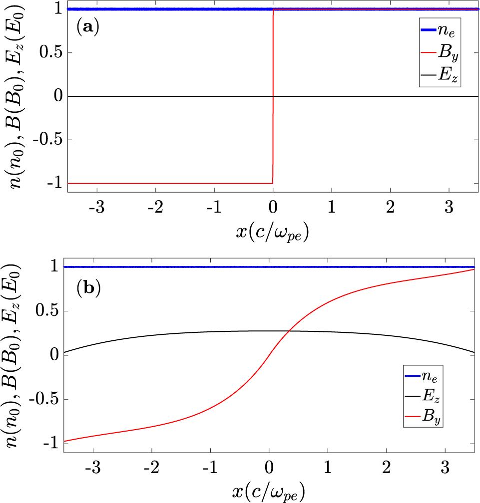
    Figure 1.(a) The initial condition of 1D model. (b) Magnetic field annihilation and electric field growing.

    The expected electric field growing is shown in Figure 1(b). The strength of magnetic field significantly decreases near the critical point of $x=0$ and ${E}_z$ grows in the corresponding region with a transverse expansion along $x$-direction. Notice that such magnetic annihilation and electric field generation are valid in both highly-conducting collisional and collisionless plasmas and even in the vacuum. In this review, the magnetic annihilation and reconnection in the collisionless plasmas are focused.

    2.2 Finite amplitude opposite polarity electromagnetic wave interaction with thin current layer

    Now we consider the finite amplitude electromagnetic wave collision with the electric current carrying thin plasma layer. This current sheet in the $yz$ plane has the electric current density described by the expression

    $$\begin{align}\mathbf{j}={I}_0\delta (x){\mathbf{e}}_z={n}_0 lc\delta (x){\mathbf{e}}_z\sum \limits_{j=e,i}{e}_j\frac{p_{j,0}}{\sqrt{m_j^2{c}^2+{p}_{0,j}^2}}.\end{align}$$ 

    An electromagnetic wave of amplitude ${E}_w$, given at $t<0$ by the electromagnetic potential $\mathbf{A}=-{E}_w\left( ct+|x|\right)\cdot \theta ( ct+|x|){\mathbf{e}}_z$, is incident on the current sheet. The equation for the field (4) takes the form

    $$\begin{align}&{c}^2{\partial}_{tt}a-{\partial}_{xx}a=-2{\omega}_{0e}\delta (x)\notag\\&\quad\times{}\left[\frac{a+{\pi}_e}{\sqrt{1+{\left(a+{\pi}_e\right)}^2}}+\mu \frac{a-{\pi}_i}{\sqrt{1+{\mu}^2{\left(a-{\pi}_i\right)}^2}}\right]\notag\\&\quad{}+\frac{2e}{m_e{c}^2}\left({E}_w+{B}_0\right){\delta}^{\prime }(t)+\frac{2e}{m_e}{E}_w\delta (t),\end{align}$$ 

    where

    $$\begin{align}{\omega}_{0e}=\frac{2\pi {n}_0{e}^2l}{m_ec},\end{align}$$ 

    the normalized field equals $a={eA}_z/{m}_e{c}^2$, the normalized initial electron and ion momenta are ${\pi}_e={p}_{e,0}/{m}_ec$ and ${\pi}_i={p}_{i,0}/{m}_ec$, respectively, and $\mu ={m}_e/{m}_p$ is the electron to ion mass ratio. We assume that ${m}_i={m}_p$.

    Equation (12) can be written by using the d’Alembert relationship, giving the solution of the Cauchy problem for the wave equation, as

    $$\begin{align}&a\left(x,t\right)=\notag\\&\quad{}-{\omega}_{0e}{\int}_0^{t-\mid x\mid /c}\left\{\frac{a\left(0,{t}^{\prime}\right)+{\pi}_e}{\sqrt{1+{\left[a\left(0,{t}^{\prime}\right)+{\pi}_e\right]}^2}}\right.\notag\\&\quad{}\!\left.+\mu \frac{a\left(0,{t}^{\prime}\right)-{\pi}_i}{\sqrt{1+{\mu}^2{\left[a\left(0,{t}^{\prime}\right)-{\pi}_i\right]}^2}}\right\}\hbox{d}{t}^{\prime}\notag\\&\quad{}+\frac{2\pi {eI}_0}{m_e{c}^2}[\mid\! x\!\mid +\theta ( ct-|x|)( ct-|x|)]\notag\\&\quad{}-\frac{eE_w}{m_e{c}^3}\left[\left( ct+x\right)\theta\! \left( ct+x\right)+\left( ct-x\right)\theta\! \left( ct-x\right)\right].\end{align}$$ 

    To find the function $a\left(0,t\right)$ we set $x=0$ in Equation (14) and differentiate it with respect to time $t$. The result is an ordinary differential equation of the first order whose solution is

    $$\begin{align}&{\int}_0^a\left(0,t\right)\left[\frac{a^{\prime }+{\pi}_e}{\sqrt{1+{\left({a}^{\prime }+{\pi}_e\right)}^2}}+\mu \frac{a^{\prime }-{\pi}_i}{\sqrt{1+{\mu}^2{\left({a}^{\prime }-{\pi}_i\right)}^2}}\right.\notag\\&\quad{}{\left.-\frac{2\pi {eI}_0}{m_e{c}^2{\omega}_{0e}}-\frac{2{eE}_w}{m_e{c}^2{\omega}_{0e}}\right]}^{-1}\hbox{d}{a}^{\prime }=-{\omega}_{0e}t.\end{align}$$ 

    One may see from Equation (15) that if the amplitude of the electromagnetic wave is substantially large, ${E}_w>4\pi {en}_0l-\pi {I}_0/c$, there can be no steady state solution. In the limit $t\to \infty$ the electromagnetic potential at $x=0$ grows proportionally to time as

    $$\begin{align}a\left(0,t\right)\approx -\frac{et}{m_ec}\left[{E}_w-\frac{\pi }{c}\left(4{en}_0 lc-{I}_0\right)\right].\end{align}$$ 

    Consequently, the unlimited acceleration of charged particles occurs with the particle momentum growing as

    $$\begin{align}{p}_z\left(0,t\right)\approx - et\left[{E}_w-\frac{\pi }{c}\left(4{en}_0 lc-{I}_0\right)\right].\end{align}$$ 

    Substituting the function $a\left(0,t\right)$ found from Equation (15) to (14) we obtain the expression describing the electromagnetic field outside the current sheet. In the case of super-strong electromagnetic field, when ${E}_w>4\pi {en}_0l-\pi {I}_0/c$, the electric field has a form of two almost constant waves with the amplitude ${E}_w-4\pi {en}_0l+\pi {I}_0/c$ propagating outwards in two directions. For the electromagnetic wave incident on the current sheet with moderate amplitude, ${E}_w<4\pi {en}_0l-\pi {I}_0/c$, the wave is reflected from the current sheet. In the region $\mid x\mid < ct$ the electric field vanishes and the magnetic field is equal to ${B}_y=\left({B}_0+{E}_w\right)\operatorname{sgn}(x)$. The momentum of charged particles increases a finite value.

    We note that the solution found here corresponds to the paradigm of the thin foil nonlinear electrodynamics developed in Refs. [89,9194].

    2.3 Tearing mode instability of thin current layer

    The 2D dynamics of thin current sheet is considered within the framework of the tearing mode instability concept. The electromagnetic tearing mode instability of thin current sheet has been studied in Refs. [37,89,9597]. The electromagnetic field given by the vector $\mathbf{A}=\left({m}_e{c}^2a/e\right){\mathbf{e}}_z$ and electrostatic potential $\varphi ={m}_e{c}^2\phi /e$ is governed by the equations

    $$\begin{align}{W} a=\delta (x)J,\end{align}$$ 

    $$\begin{align}{W} \varphi =\delta (x)R,\end{align}$$ 

    where ${W} ={\partial}_{xx}+{\partial}_{yy}-{c}^{-2}{\partial}_{tt}$ is the d’Alambertian,

    $$\begin{align}J=4\pi \sum \limits_{j=e,i}{e}_j{n}_j{lv}_{z,j}/{m}_j{c}^2\end{align}$$ 

    and

    $$\begin{align}R=4\pi \sum \limits_{j=e,i}{e}_j{n}_jl/{m}_j{c}^2\end{align}$$ 

    are the surface electric current and electric charge density, respectively. Here it is assumed that the variables $a$ and $\varphi$ depend on the coordinates $x$, $y$ and time $t$. Linearizing Equations (18) and (19) and presenting dependence of the potentials on time and coordinates in the form ${a}^{(1)}={a}^{(1)}(x)\exp \left(-\omega t+ ikx\right)$ and ${\varphi}^{(1)}={\varphi}^{(1)}\exp \left(-\omega t+ ikx\right)$, we can write the Equations (18) and (19) as

    $$\begin{align}\frac{\hbox{d}^2{a}^{(1)}}{\hbox{d}x^2}-{Q}^2{a}^{(1)}=\delta (x)\left({J}_a{a}^{(1)}+{J}_{\varphi }{\varphi}^{(1)}\right),\end{align}$$ 

    $$\begin{align}\frac{\hbox{d}^2{\varphi}^{(1)}}{\hbox{d}x^2}-{Q}^2{\varphi}^{(1)}=\delta (x)\left({R}_a{a}^{(1)}+{R}_{\varphi }{\varphi}^{(1)}\right),\end{align}$$ 

    with ${J}_a={\partial}_aJ$, ${J}_{\varphi }={\partial}_{\varphi }J$, ${R}_a={\partial}_aR$, and ${R}_{\varphi }={\partial}_{\varphi }R$, where

    $$\begin{align}Q=\sqrt{k^2-{\omega}^2/{c}^2}.\end{align}$$ 

    The solution of Equations (22) and (23) yields

    $$\begin{align}{a}^{(1)}(x)=-\frac{\exp \left(-Q|x|\right)}{2Q}\left[{J}_a{a}^{(1)}(0)+{J}_{\varphi }{\varphi}^{(1)}(0)\right],\end{align}$$ 

    $$\begin{align}{\varphi}^{(1)}(x)=-\frac{\exp \left(-Q|x|\right)}{2Q}\left[{R}_a{a}^{(1)}(0)+{R}_{\varphi }{\varphi}^{(1)}(0)\right].\end{align}$$ 

    Setting $x=0$ in both sides of Equations (25) and (26) we obtain the system of algebraic equations. The condition of solvability of the system obtained results in the equation

    $$\begin{align}1+\frac{J_a+{R}_{\varphi }}{2Q}+\frac{J_a{R}_{\varphi }-{R}_a{J}_{\varphi }}{4{Q}^2}=0.\end{align}$$ 

    We assume that the unperturbed electric current density and electric charge density are ${J}^{(0)}=-4\pi {en}_e^{(0)}{lv}_{z,e}^{(0)}/c$ and ${R}^{(0)}=0$, respectively. Here the electron velocity along the $z$ axis is ${v}_{z,e}^{(0)}={\beta}_0c$.

    Obtained within the framework of cold electron and ion hydrodynamics approximation ${J}_a$, ${J}_{\varphi }$, ${R}_a$, and ${R}_{\varphi }$ are given by

    $$\begin{align}{J}_a=\frac{2{\omega}_{0e}}{c}\left(\frac{1}{\gamma^{(0)3}}+\mu +\frac{k^2{c}^2}{\omega^2{\gamma}^{(0)}}{\beta}^{(0)}\right),\end{align}$$ 

    $$\begin{align}{J}_{\varphi }=-\frac{2{\omega}_{0e}}{c}\frac{k^2{c}^2}{\omega^2{\gamma}^{(0)}}{\beta}^{(0)},\end{align}$$ 

    $$\begin{align}{R}_a=\frac{2{\omega}_{0e}}{c}\frac{k^2{c}^2}{\omega^2{\gamma}^{(0)}}{\beta}^{(0)},\end{align}$$ 

    $$\begin{align}{R}_{\varphi }=-\frac{2{\omega}_{0e}}{c}\frac{k^2{c}^2}{\omega^2}\left(\frac{1}{\gamma^{(0)}}+\mu \right),\end{align}$$ 

    with ${\gamma}^{(0)}=1/\sqrt{1-{\beta}^{(0)2}}$. Substituting these expressions for ${J}_a$, ${J}_{\varphi }$, ${R}_a$, and ${R}_{\varphi }$ into Equation (27) we obtain the dispersion equation for the frequency $\omega$ and wave number $k$. It is

    $$\begin{align}&{W}^2\left[1+\frac{\omega_{0e}}{Qc}\left(\frac{1}{\gamma^{(0)3}}+\mu \right)\right]+W\frac{\omega_{0e}}{Qc}\left[\frac{\beta^{(0)2}}{\gamma^{(0)2}}\right.\notag\\&\quad{}\left.-\frac{1}{\gamma^{(0)}}-\mu -\frac{\omega_{0e}}{Qc}\left(\frac{1}{\gamma^{(0)3}}+\mu \right)\left(\frac{1}{\gamma^{(0)}}+\mu \right)\right]\notag\\&\quad{}-{\left(\frac{\omega_{0e}}{Qc}\right)}^2\frac{{\mu \beta}^{(0)2}}{\gamma^{(0)2}}=0,\end{align}$$ 

    where $W={\left(\omega / kc\right)}^2$.

    In the short wavelength limit, when $kc/{\omega}_{0e} \gg 1$ the growth rate of the tearing instability is approximately equal to

     (33)

    In the long wavelength limit, when $kc/{\omega}_{0e}\ll 1$ we have the growth rate of the tearing instability

     (34)

    For high enough electron energy, in the range ${\mu}^{-1}\gg {\gamma}^{(0)}\gg {\mu}^{-1/3}$, does not depend on the electron to ion mass ratio, $\mu$, being approximately equal to $kc{\beta}^{(0)}{\gamma}^{(0)}$.

    Following from Equation (33) in the non-relativistic limit, when ${\beta}^{(0)}\ll 1$ and ${\gamma}^{(0)}\approx 1$, the growth rate of the tearing mode instability of thin current sheet is $kc{\beta}^{(0)}\sqrt{\mu }$ (see also Ref. [89]).

    2.4 The electric and magnetic field configuration arising during decay of thin current sheet

    In the case of a thin current sheet localized in the $y=0$ plane carrying the surface electric current density $2{en}_0 lc{\beta}^{(0)}\delta (y)$, the magnetic field produced by this current is $\mathbf{B}=\left({B}_0\kern0.1em \operatorname{sgn}(x),\mathrm{0,0}\right)$ with ${B}_0=4\pi {en}_0 lc{\beta}^{(0)}$. At the nonlinear stage of the tearing mode thin current sheet can break forming a finite length hole in the density distribution[97]. Accordingly, it is worthwhile to analyze in detail the electromagnetic field configuration which arise during the current sheet decay. Here we examine a model for the current sheet decay assuming the time evolution of the electric current to be given: at $t>0$ the electric current density is described by the dependence

    $$\begin{align}\mathbf{j}&={I}_0f\left(x,t\right)\delta (y){\mathbf{e}}_z,\notag\\f\left(x,t\right)&=1-\theta \left[x(t)-|x|\right].\end{align}$$ 

    In other words the current sheet breaks into halves, which move apart along the $x$ axis with their ends coordinates given by $x=\pm x(t)$, i.e., the width of the gap formed in the current sheet increases as $2x(t)$.

    The electromagnetic field (it is the normalized electromagnetic potential $a={eA}_z/{m}_e{c}^2$) is described by the wave equation

    $$\begin{align}{\partial}_{xx}a+{\partial}_{yy}a-{c}^{-2}{\partial}_{tt}a=-\frac{\omega_{0e}}{c}{I}_0f\left(x,t\right)\delta (y)\end{align}$$ 

    with the initial conditions

    $$\begin{align}&a\left(t=0\right)=-\frac{\omega_{0e}}{c}\mid y\mid,&{\partial}_ta\left(t=0\right)=0.\end{align}$$ 

    Solving the Cauchy problem for Equations (36) and (37) with the surface electric current density given by Equation (35), we find the electric field ${E}_z=-{\partial}_t{A}_z/c$ and magnetic field ${B}_y=-{\partial}_x{A}_z/c$ (the normalized fields equal $d={eE}_z/{m}_ec=-\dot{a}$ and $b={eB}_y/{m}_ec=-{a}^{\prime }$). Here and below dot and prime stand for derivatives with respect to time and $x$ coordinate.

    Contours of equal value of the electric field in the xy plane at .

    Figure 2.Contours of equal value of the electric field in the xy plane at .

    The $y$ component of the magnetic field is given by

    $$\begin{align}&{B}_y\left(x,y,t\right)=\frac{I_0}{2c\sqrt{1-{\beta}^2}}\notag\\&\quad{}\times \ln \left[\frac{\left({t}_{+}+\sqrt{t^2-{r}^2/{c}^2}\right)\left({t}_{-}-\sqrt{t^2-{r}^2/{c}^2}\right)}{\left({t}_{+}-\sqrt{t^2-{r}^2/{c}^2}\right)\left({t}_{-}+\sqrt{t^2-{r}^2/{c}^2}\right)}\right].\end{align}$$ 

    The $x$ component of the magnetic field vanishes in the plane $y=0$ due to symmetry of the problem under consideration.

    At the point $r=0$ the magnetic field is equal to zero, ${B}=0$, for all $t$. The electric field here is constant, given by

    $$\begin{align}{E}_z\left(r=0,t\right)=\frac{I_0\beta }{c\sqrt{1-{\beta}^2}}\ln \left(\frac{1+\sqrt{1-{\beta}^2}}{1-\sqrt{1-{\beta}^2}}\right).\end{align}$$ 

    In the non-relativistic limit of the current sheet evolution for $\beta = 1$ the electric field is

    $$\begin{align}{E}_z\left(r=0,t\right)\approx \frac{2{I}_0\beta }{c}\ln \left(\frac{2}{\beta}\right).\end{align}$$ 

    In the ultra-relativistic case, with $\beta \to 1$, we have the electric field ${E}_z\left(r=0,t\right)\approx 4{I}_0$.

    In the vicinity of the point $r=0$ the magnetic field is a linear function of the coordinates. According to Equation (41) here the magnetic field is

    $$\begin{align}{B}_y\left(r=0,t\right)\approx \frac{4{I}_0}{c\beta t}x.\end{align}$$ 

    We see that the electric field $E\approx \beta {B}_0$ is generated as the current sheet decays. Here ${B}_0$ is the magnetic field far outside of the current sheet and $\beta =v/c$ with $v$ equal to the characteristic plasma velocity.

    Using the relationships obtained above for the electric and magnetic fields near the point $r=0$ (i.e., in the region $r<\beta ct$) the electromagnetic potential can be approximated as

    $$\begin{align}{A}_z\left(x,y,t\right)\approx -\frac{1}{\pi }{B}_0\beta ct+\frac{B_0}{\pi \beta ct}\left({x}^2-{y}^2\right).\end{align}$$ 

    This expression describes nonstationary zero line of the magnetic field of hyperbolic type. The electric field directed along the zero line is constant, while the gradient of the magnetic field decreases inversely proportional to the time.

    3 Spontaneous magnetic field generation in laser-plasma interaction

    3.1 Thermoelectric field and ponderomotive driven field

    Considering unmagnetized plasmas with ideal MHD condition, the electrons move quickly along the temperature and density gradients due to their small inertia. The non-neutral charge distribution generates an electric field. Combine the ideal Ohm’s law (Equation (46)) and Cauchy momentum Equation (47),

    $$\begin{align}\mathbf{E}+\frac{\mathbf{u}\times \mathbf{B}}{c}=0,\end{align}$$ 

    $$\begin{align}{n}_e{m}_e{\partial}_t\mathbf{u}=\frac{\mathbf{j}\times \mathbf{B}}{c}-\nabla P,\end{align}$$ 

    where $P$ is the electron pressure and ${n}_e$ is the number density of the electron component. Taking the quasi-stationary condition (${\partial}_t\mathbf{u}=0$) into account, the self-generated electric field is obtained,

    $$\begin{align}\mathbf{E}=-\frac{\nabla P}{en_e}.\end{align}$$ 

    Such a field is the response of the plasma to prevent the electrons motion according to the gradients in electron pressure. Applying curl on Equation (48) and plugging in Faraday’s law (Equation (9)), it yields

    $$\begin{align}{\partial}_t\mathbf{B}=-c\frac{\nabla {n}_e\times \nabla P}{en_e^2}.\end{align}$$ 

    Using the equation of state,

    $$\begin{align}P={n}_e{k}_B{T}_e,\end{align}$$ 

    Equation (49) can be further extended to

    $$\begin{align}{\partial}_t\mathbf{B}=-\frac{ck_B}{en_e}\left(\nabla {n}_e\times \nabla {T}_e\right),\end{align}$$ 

    where ${k}_B$ is the Boltzmann constant and ${T}_e$ is the electron temperature. When the laser irradiates on the solid surface, the density varies mainly along the longitudinal direction and the temperature gradient is significant in the transverse direction. Therefore, a toroidal magnetic field is generated around the laser axis due to the misalignment between the gradients of the density and temperature. Such a spontaneous magnetic field generation process is often called as the Biermann battery effect[51]. It is proposed to be the origin source of magnetic field in astrophysics and amplified as the seed fields[98]. Biermann battery effect has also been applied in the early laser driven MR experiments[50,52] with moderate intensities (${\sim}{10}^{15}\ \mathrm{W}/{\mathrm{cm}}^2$) and long pulse length (${\sim} \hbox{ns}$), mega-gauss magnetic fields in plasmas at the focal spot edges were obtained.

    When the laser intensity becomes higher, the ponderomotive force of the laser field expels the electrons away from the focal spot and significantly changes the local density distributions forming sharp density gradients. By the continuous radiation pushing, the background electrons are prevented from returning and shielding against the charge separation field. A ponderomotive electric current is formed $\mathbf{J}={n}_ee\mathbf{v}\sim {n}_e\nabla I$ and it induces the magnetic field as $\textbf{B}\sim \nabla {n}_e\times \nabla I$. Theoretical and numerical studies have proved that magnetic field with 100 MG can be generated via the interaction of overdense plasma and intense ($\mathit{I}\sim {10}^{18}\ \mathrm{W}/{\mathrm{cm}}^2$) laser pulse[99103]. Comparing with Biermann battery effect, the ponderomotive driven magnetic field is much stronger. However, it decays quickly after the laser-matter interaction, which indicates the field has a life time with the scale of the pulse duration ($t\sim {\tau}_L$). In contrast, the magnetic field in Bierman battery effect decays in a long time scale and can be regarded as a quasi-steady field.

    3.2 Static magnetic field driven by energetic electron beam

    The generation of magnetic field based on ultra intense laser-plasma interactions has been investigated intensively in recent years[104106]. Furthermore, the interactions of beam-plasma are also discussed for strong magnetic dipoles generation[107,108]. The magnetic field generation under the condition of ultra-intense laser interacting with underdense or near critical density plasma is discussed in this section. The ultra-intense laser considered here means the corresponding intensity exceeds the relativistic threshold ($I\gg {10}^{18}\ \mathrm{W}/{\mathrm{cm}}^2$) and the laser power is beyond the characteristic power of self-focusing (${\mathcal{P}}_c=2{m}_e^2{c}^5/{e}^2=17\ \mathrm{GW}$)[109]. The laser is assumed to have a short pulse duration ($c{\tau}_L\sim {\lambda}_p$), in which ${\lambda}_p$ is the plasma wavelength.

    The strong ponderomotive force quickly expels electrons from the laser path and leaves an electron plasma channel which has a positive charge background since ions with heavier inertia response slowly. Balancing the electron energy gain and loss from the laser and the electrostatic potential,

    $$\begin{align}e{\phi}_{static}={\varepsilon}_{pond},\end{align}$$ 

    $$\begin{align}\pi {n}_e{e}^2{R}_{ch}^2={a}_{ch}{m}_e{c}^2,\end{align}$$ 

    the radius of the plasma channel can be estimated,

    $$\begin{align}{R}_{ch}=\sqrt{\frac{a_{ch}{n}_c}{n_e}}\frac{\lambda }{\pi },\end{align}$$ 

    where ${n}_c=m{\omega}_L^2/4\pi {e}^2$ is the critical density of plasmas and $\lambda$ is the laser wavelength. ${a}_{ch}$ is the laser pulse amplitude inside the plasma channel[110], which is proportional to the laser power and plasma density,

    $$\begin{align}{a}_{ch}={\left(\frac{2}{K}\frac{\mathcal{P}}{{\mathcal{P}}_c}\frac{n_e}{n_c}\right)}^{1/3},\end{align}$$ 

    where $K$ is a constant factor coming from the integration over the duration of the laser pulse.

    The charge separation field in the plasma channel appears at the wake of the laser pulse and forms the so-called wakefield[111]. In a relatively low density collisionless plasma, the induced wakefield, following the laser pulse, propagates with a phase velocity close to the speed of light in vacuum. The electrons injected into the acceleration phase of the wakefield with the initial velocity close to the wakefield phase velocity can be trapped and accelerated. The strength of the wakefield behind the laser pulse has been analytically studied[112],

    $$\begin{align}{E}_x\left(\zeta, r\right)=-\frac{2{\pi}^2{k}_p{\phi}_L(r)}{4{\pi}^2-{k}_p^2{\left(c{\tau}_L\right)}^2}\times \left[\sin {k}_p\left(c{\tau}_L-\zeta \right)+\sin {k}_p\zeta \right],\end{align}$$ 

    where the laser is supposed to propagate in $x$-direction, $\zeta =x- ct$ is the transformation to the light frame, ${\phi}_L$ is the ponderomotive potential of the laser pulse, and ${k}_p=2\pi /{\lambda}_p$ is the wave number of the Langmuir waves.

    The trapped and accelerated electron beam generates a current along the plasma channel. In the case of near critical density plasma, the accelerated beam contains a large electric charge resulting in a strong direct current. Consequently, the azimuthal magnetic field confined in the plasma channel is produced. From Ampere-Maxwell law,

    $$\begin{align}\nabla \times \mathbf{B}=\frac{4\pi }{c}\mathbf{j}+\frac{1}{c}{\partial}_t\mathbf{E},\end{align}$$ 

    the strength of the magnetic field can be estimated provided the quasi-static condition of ${\partial}_t\mathbf{E}=0$. Since the magnetic field has the same size as the radius of the plasma channel, one obtains the maximum amplitude,

    $$\begin{align}\mid \mathbf{B}\mid =4\pi {n}_e{eR}_{ch}.\end{align}$$ 

    An example of kinetic simulation is presented here to demonstrate the details of the process. Linear polarized laser with the intensity ${I}_0={10}^{21}\ \mathrm{W}/{\mathrm{cm}}^2$ is incident into the plasma target with the peak density of ${n}_e=0.25{n}_c$ and propagates along $x$-direction. The laser pulse has Gaussian profiles in both transverse and longitudinal directions with the full width at half maximum (FWHM) spot size of and pulse duration ${\tau}_L=30\ \mathrm{fs}$.

    The numerical demonstration of static magnetic field driven by energetic electron beam. (a) The electron density distribution with the plasma channel formation. (b) The blue and red curves represent the longitudinal electric field and the electron density profile on the laser axis (). (c) The average energy distribution of the electrons. (d) The z component of the azimuthal magnetic field induced by the energetic electron beam.

    Figure 3.The numerical demonstration of static magnetic field driven by energetic electron beam. (a) The electron density distribution with the plasma channel formation. (b) The blue and red curves represent the longitudinal electric field and the electron density profile on the laser axis (). (c) The average energy distribution of the electrons. (d) The z component of the azimuthal magnetic field induced by the energetic electron beam.

    The profile of the longitudinal electric field along the laser axis ($y=0$) is presented in Figure 3(b) and the maximum of the acceleration phase reaches about ${E}_{x,\mathit{\max}}\approx 65\ \mathrm{GV}/\mathrm{cm}$. The corresponding electron density profile (blue in Figure 3(b)) indicates a bunch of the electrons are trapped and accelerated in the wakefield. With such a high acceleration gradient, the electrons in the channel are expected to gain energy quickly. The average energy distribution of the electrons,

    $$\begin{align}<{\varepsilon}_e>=\frac{\int {\varepsilon}_e\left(x,y\right)f\left(x,y\right) \hbox{d}x\hbox{d}y}{\int f\left(x,y\right) \hbox{d}x\hbox{d}y},\end{align}$$ 

    is shown in Figure 3(c). The energy of the electron beam reaches hundreds MeV and it corresponds to an electric current density of $\approx 0.2{n}_c ec$. According to Ampere-Maxwell law, an azimuthal magnetic field is generated with the same radius of the plasma channel as presented in Figure 3(d). The amplitude reaches about 0.6 GG which agrees with the estimate obtained from Equation (58). The magnetic dipole propagates together with the laser pulse in the plasma channel, which is quasi-steady till the laser depletion and the electron beam dissipation. The depletion length of the pumping laser can be estimated when the laser energy is completely dumped to the excited wakefield (${\varepsilon}_L\sim {\varepsilon}_w$),

    $$\begin{align}\frac{E_L^2}{4\pi }c{\tau}_L={n}_e{m}_e{c}^2\frac{a_{ch}^2}{2}{l}_{dp},\end{align}$$ 

    which can be rewritten in the form of

    $$\begin{align}{l}_{dp}=\frac{2c{\tau}_L}{a_0^2}{\left(\frac{2}{K}\frac{\mathcal{P}}{{\mathcal{P}}_c}\frac{\omega_0}{\omega_{pe}}\right)}^{2/3}.\end{align}$$ 

    Equation (62) indicates that the magnetic field has a relatively long time scale in the ultra-intense laser case, which is important for designing the corresponding experiment.

    4 Relativistic MR and magnetic field energy dissipation

    4.1 Magnetic dipole expansion

    (a) The transverse expansion of the magnetic dipole along a density downramp region. The distributions of at different snapshots are combined here. (b) The profiles of along different -coordinates.

    Figure 4.(a) The transverse expansion of the magnetic dipole along a density downramp region. The distributions of at different snapshots are combined here. (b) The profiles of along different -coordinates.

    The expansion of the magnetic dipole in the density downramp provides an optimal condition for the study of MR. By sending two parallel identical laser pulses into the plasma (laser axes distributed at ${y}_1$ and ${y}_2$ along $y$-direction), a pair of azimuthal magnetic dipoles are generated by the parallel accelerated electron beams. In the ideal case, the two magnetic dipoles are translational symmetry along the transverse direction,

    $$\begin{align}\mathbf{B}\left(x,y,z\right)=\mathbf{B}\left(x,y+d,z\right),\end{align}$$ 

    where $d$ is the separation distance of the two laser axes. It should be noted that the separation distance between the two pulses should be large enough to avoid the two plasma channels interference with each other in the initial stage, i.e., $d>2{R}_{ch}$. Due to the feature of magnetic dipole in each channel, the total magnetic field has an antisymmetry distribution on the two sides of the system center ${y}_c=\left({y}_1+{y}_2\right)/2$, i.e.,

    $$\begin{align}\mathbf{B}\left(x,{y}_c+y,z\right)=-\mathbf{B}\left(x,{y}_c-y,z\right).\end{align}$$ 

    Therefore, with the expansion of the two magnetic dipoles, the opposite magnetic polarities approach at the central region in transverse, where the magnetic field annihilation and the field line reconnection are expected to occur.

    (a) The energy density distribution () of electrons. The round circles represent the azimuthal magnetic fields. The projections of components in (b) the uniform density region and (c) the density downramp region.

    Figure 5.(a) The energy density distribution () of electrons. The round circles represent the azimuthal magnetic fields. The projections of components in (b) the uniform density region and (c) the density downramp region.

    4.2 Magnetic field annihilation and field line reconnection

    The 2D magnetic configuration in the transverse plane ($yz$ plane) can be described by a complex function[115],

    $$\begin{align}B\left(y,z\right)={B}_y-{iB}_z,\end{align}$$ 

    with a complex variable $\zeta =y+ iz$. In the vicinity of the reconnection region (the dashed line in Figure 5(c)), the magnetic field lines form a hyperbolic structure in the transverse plane and the constant potential surface is

    $$\begin{align}\mid \mathbf{A}\left(y,z\right)\mid =\Re \left\{{B}_0{\zeta}^2/2\right\}.\end{align}$$ 

    (a) and (b) are contours of the constant vector potentials around the -point based on theoretical model. (a) refers to the initial stage when the opposite magnetic fields just begin to vanish. (b) refers to the moment when the current sheet in MR has formed and bifurcated. (c) and (d) are the corresponding distributions demonstrated by numerical simulations.

    Figure 6.(a) and (b) are contours of the constant vector potentials around the -point based on theoretical model. (a) refers to the initial stage when the opposite magnetic fields just begin to vanish. (b) refers to the moment when the current sheet in MR has formed and bifurcated. (c) and (d) are the corresponding distributions demonstrated by numerical simulations.

    Therefore the charged particles can be accelerated during MR via such an electric field produced by the rapid change of magnetic field, which will be discussed in detail in the next section. The current driven by the accelerated particles generates an extra magnetic field represented by the blue curve in Figure 6(b). The new magnetic field changes the field topology and the $X$-point breaks into two new zeroth points as depicted by ${X}^{\prime }$. The $X$-point bifurcation continues and the $X$-point grows to be a current layer shown by the red region in Figure 6(b), which is known as the current sheet. It can also be understood as the electric current filamentation and breaks up to separated pieces due to the tearing mode instability. The development of such a process takes about 15 laser periods. According to the theoretical estimate in Equation (33) under the short wavelength limit, the growth rate of the tearing instability is about ${\tau}^{-1}$, the reciprocal of the pulse duration, which is about 11 laser periods. The broken configuration of magnetic field is given by

    $$\begin{align}B\left(y,z\right)=\frac{B_0\zeta }{\sqrt{s{(t)}^2-{\zeta}^2}}.\end{align}$$ 

    Here $s$ is the spatial scale of current sheet modulation[115,116]. The corresponding vector potential is

    $$\begin{align}\mid \mathbf{A}\left(y,z\right)\mid =\Re \left\{{B}_0\sqrt{s{(t)}^2-{\zeta}^2}\right\}.\end{align}$$ 

    Recalling Equation (70), the electric field is given as

    $$\begin{align}E(t)=-\frac{1}{c}\frac{B_0s(t)\dot{s}(t)}{\sqrt{s{(t)}^2-{\zeta}^2}}.\end{align}$$ 

    The 2D configuration of magnetic field lines and the constant vector potential is demonstrated by a 3D numerical simulation. The curves and the vectors in Figures 6(c) and 6(d) present the contour magnetic field strength and the magnetic field lines with directions. The formation of $X$-point corresponding to the situation of Figure 6(a) is shown in Figure 6(c) in which the magnetic field loops produced by the parallel currents form an eight-like curve with a single zeroth-point localized in the center. The opposite magnetic field lines in the vicinity of the zeroth-point are not vanishing each other at this moment.

    With the process of MR and the development of tearing instability, the $X$-point breaks and a thin current sheet grows as seen in Figure 6(d). The new closed loops in the middle of the current sheet can be regarded as the magnetic islands which are the results of tearing driven current filamentation. The $X$-point also separates along $z$-direction and the magnetic field lines around the bifurcated ${X}^{\prime}$-points change their directions to connect the lines generated from the other current (indicated by the vectors). The evolution of the magnetic field structures shown in Figure 6(d) is well consistent with the theoretical model displayed in Figure 6(b).

    4.3 Relativistic magnetic field dissipation and inductive electric field generation

    Recalling Ampere-Maxwell law in Equation (57), the term of displacement current (${\mathbf{j}}_D={\partial}_t\mathbf{E}$) is normally neglected in the context of MHD approximation. In the vicinity of the current sheet, the curl of magnetic field can be estimated as $B/{r}_{cs}$, where ${r}_{cs}$ is the characteristic size of the current sheet. In this case, the Ampere-Maxwell equation excluding displacement current can be rewritten as

    $$\begin{align}\frac{B}{r_{cs}}=\frac{4\pi }{c}{n}_{cs} eu,\end{align}$$ 

    where ${n}_{cs}$ and $u$ are the density and velocity of the charged particles inside current sheet. Due to the relativistic constraint that the particle velocity cannot exceed the speed of light, the following relation is obtained to satisfy the MHD approximation,

    $$\begin{align}\frac{B}{4\pi {en}_{cs}{r}_{cs}}=\frac{u}{c}\le 1.\end{align}$$ 

    However, in the relativistic regime of MR, such a relation is not always satisfied. Considering the situation of ultra-intense laser interacting with underdense or near critical density plasma, substituting the magnetic field with Equation (58), one obtains

    $$\begin{align}\frac{n_e{R}_{ch}}{n_{cs}{r}_{cs}}=\frac{u}{c}\approx 1.\end{align}$$ 

    Here the velocities of the relativistic charged particles are assumed to reach their upper limits of the light speed. As mentioned above, the current sheet is formed in the density downramp region where the magnetic dipoles are expanding, which implies the local density is much lower than the density plateau where the energetic electron beams and static magnetic fields are formed, i.e., ${n}_{cs}\ll {n}_e$. On the other hand, the size of the current sheet is obviously smaller than the radius of magnetic dipoles, i.e., ${r}_{cs}\ll {R}_{ch}$. Therefore, under the relativistic MR regime, the above relation changes to

    $$\begin{align}\frac{n_e{R}_{ch}}{n_{cs}{r}_{cs}}\gg 1,\end{align}$$ 

    and the restrained condition for MHD approximation in Equation (75) becomes invalid. This means the limited conduction current (${n}_e ec$) is not able to sustain the variation of magnetic field ($\nabla \times B$) and the effect of the displacement current (${j}_D={\partial}_tE$) must be taken into account. The displacement current refers to the growth rate of an inductive electric field. To compensate the difference of $c\nabla \times B$ and the conduction current, substituting magnetic field with Equation (58) and the local current in the current sheet with ${n}_{cs} ec$, the inductive electric field is obtained,

    $$\begin{align}{\partial}_tE=4\pi {n}_e ec\left(\frac{R_{ch}}{r_{cs}}-\frac{n_{cs}}{n_e}\right).\end{align}$$ 

    The displacement current plays an important role here to balance the fast magnetic field variation and converts the energy from magnetic field to electric field. The growing inductive electric field indicates the relativistic MR is a non-stationary process violating the freezing-in condition and the corresponding Ohm law should be modified[73,74]. Due to the non-stationary feature, the relativistic MR is also proposed as dynamic dissipation of magnetic field[75].

    (a) The magnetic field distributions in the simulation when MR is occurring. (b) The surface represents the distribution of longitudinal electric field (). The curves are the profiles of all the components in Ampere-Maxwell law (Equation (57)).

    Figure 7.(a) The magnetic field distributions in the simulation when MR is occurring. (b) The surface represents the distribution of longitudinal electric field (). The curves are the profiles of all the components in Ampere-Maxwell law (Equation (57)).

    4.4 Charged particle acceleration in relativistic MR

    The energy distributions of the electrons inside current sheet before and after magnetic field reconnection.

    Figure 8.The energy distributions of the electrons inside current sheet before and after magnetic field reconnection.

    (a) Schematic of the theoretical model in the vicinity of -point. (b) The analytical solutions of particles motion with the expressions in Equations (96) and (97). (c) and (d) are the trajectories of charged particles given by the solutions of Equations (98) and (99) for the initial conditions of , and . (e) and (f) show the typical accelerated particle trajectories obtained in the kinetic simulations.

    Figure 9.(a) Schematic of the theoretical model in the vicinity of -point. (b) The analytical solutions of particles motion with the expressions in Equations (96) and (97). (c) and (d) are the trajectories of charged particles given by the solutions of Equations (98) and (99) for the initial conditions of , and . (e) and (f) show the typical accelerated particle trajectories obtained in the kinetic simulations.

    $$\begin{align}\mathbf{B}={b}_0\left(-y\hat{\mathbf{z}}-z\hat{\mathbf{y}}\right).\end{align}$$ 

    The charged particle motion is dominated by Lorentz force $\hbox{d}\mathbf{p}/ \hbox{d}t=q\left(\mathbf{E}+\mathbf{v}\times \mathbf{B}/c\right)$. The dynamic equations for different components can be expressed as

    $$\begin{align}\frac{\hbox{d}p_x}{\hbox{d}t}={qE}_0+\frac{q}{c}{\left(\mathbf{v}\times \mathbf{B}\right)}_x=q\left[{E}_0+\frac{b_0}{2c}\frac{\hbox{d}\left({z}^2-{y}^2\right)}{\hbox{d}t}\right],\end{align}$$ 

    $$\begin{align}\frac{\hbox{d}p_y}{\hbox{d}t}=\frac{q}{c}{\left(\mathbf{v}\times \mathbf{B}\right)}_y=q\frac{b_0}{c}y\frac{\hbox{d}x}{\hbox{d}t},\end{align}$$ 

    $$\begin{align}\frac{\hbox{d}p_z}{\hbox{d}t}=\frac{q}{c}{\left(\mathbf{v}\times \mathbf{B}\right)}_z=-q\frac{b_0}{c}z\frac{\hbox{d}x}{\hbox{d}t}.\end{align}$$ 

    According to Equation (81), the particle motion in the longitudinal direction is homogeneous and can be obtained with time integral,

    $$\begin{align}{p}_x=q\left\{{E}_0t+\frac{b_0}{2c}\left[\left({z}^2-{z}_0^2\right)-\left({y}^2-{y}_0^2\right)\right]\right\}.\end{align}$$ 

    The acceleration process in MR can be derived with respect to non-relativistic and relativistic conditions[117]. Here we shall focus on the relativistic case of charged particle acceleration driven by inductive electric field. The characteristic scale length of electron motion in MR region can be estimated as the Larmor radius

    $$\begin{align}R=\frac{cp}{e\mid B\mid }=\frac{cp}{qb_0{r}_{cs}}.\end{align}$$ 

    Considering the particles are only accelerated by the longitudinal electric field,

    $$\begin{align}cp={qE}_0{r}_{cs},\end{align}$$ 

    the characteristic scale length can be written as

    $$\begin{align}R={E}_0/{b}_0,\end{align}$$ 

    and the corresponding characteristic time when the electrons are accelerated before leaving MR region is

    $$\begin{align}T=R/c={E}_0/{cb}_0.\end{align}$$ 

    The longitudinal motion of the accelerated charged particle in relativistic case is simply as

    $$\begin{align}x(t)= ct,\end{align}$$ 

    and the corresponding momentum is

    $$\begin{align}{p}_x=\gamma {mv}_x=\frac{\varepsilon \dot{\varepsilon}}{qE_0{c}^2}.\end{align}$$ 

    Here $\varepsilon$ is the kinetic energy of the particles. Comparing with the general solution of longitudinal momentum in Equation (84), one obtains

    $$\begin{align}\frac{\varepsilon \dot{\varepsilon}}{qE_0{c}^2}=q\left\{{E}_0t+\frac{b_0}{2c}\left[\left({z}^2-{z}_0^2\right)-\left({y}^2-{y}_0^2\right)\right]\right\}.\end{align}$$ 

    In the region of current sheet, where $\left({y}^2+{z}^2\right)<{R}^2$, the second term on RHS of Equation (91) can be neglected. Therefore the kinetic energy of the accelerated particles can be simplified as

    $$\begin{align}\varepsilon (t)={\left({\varepsilon}_{t=0}^2+{q}^2{E}_0^2{c}^2{t}^2\right)}^{1/2}.\end{align}$$ 

    From the equation of motion for $\hbox{d}\mathbf{p}/ \hbox{d}t=\hbox{d}\left(\gamma m\mathbf{v}/ \hbox{d}t\right)$, the following relation can be derived,

    $$\begin{align}{\ddot{x}}_{\alpha }+{\dot{x}}_{\alpha}\frac{\dot{\varepsilon}}{\varepsilon }={\dot{p}}_{\alpha}\frac{c^2}{\varepsilon },\end{align}$$ 

    here ${x}_{\alpha }$ refers to the $x$, $y$ and $z$ directions in Cartesian coordinates. Recalling Equations (82) and (83), the particle motions in the transverse plane are obtained,

    $$\begin{align}\ddot{y}+\dot{y}\frac{\dot{\varepsilon}}{\varepsilon }=-\frac{cb_0}{E_0}\frac{\dot{\varepsilon}}{\varepsilon }y,\end{align}$$ 

    $$\begin{align}\ddot{z}+\dot{z}\frac{\dot{\varepsilon}}{\varepsilon }=\frac{cb_0}{E_0}\frac{\dot{\varepsilon}}{\varepsilon }z.\end{align}$$ 

    Since the particles are accelerated to relativistic energy which is much higher than its initial energy ${\varepsilon}_{t=0}$, it is reasonable to estimate the particle kinetic energy in Equation (92) as $\varepsilon (t)={qE}_0 ct$. Therefore, the solutions of Equations (94) and (95), i.e., the particle motions in the transverse plane can be written as

    $$\begin{align}y(t)={y}_0{J}_0\left(\sqrt{\frac{4{b}_0 ct}{E_0}}\right),\end{align}$$ 

    $$\begin{align}z(t)={z}_0{I}_0\left(\sqrt{\frac{4{b}_0 ct}{E_0}}\right),\end{align}$$ 

    in which ${J}_0(x)$ and ${I}_0(x)$ are the ordinary and the modified Bessel function of zeroth order. The analytical solutions of particles motion in $y$ and $z$ directions are plotted in Figure 9(b). It presents an oscillation along $y$-direction and an exponential expansion in $z$-direction.

    In the above presented analysis of the charged particle acceleration in the vicinity of hyperbolic zero line of the magnetic field, Equations (79) and (80) describe the configuration with constant gradient of the magnetic field, i.e., ${b}_0$ is a constant. This corresponds to the case when the charged particle moves faster than the magnetic configuration changes. In ultra-relativistic limit the characteristic velocity of both the charged particles and of the magnetic field modulations is close to the speed of light in vacuum. Using Equations (44) and (71) showing that the magnetic field gradient is inversely proportional to time, ${b}_0={B}_0/\beta ct$ and $\varepsilon ={qE}_0 ct$ (see Equation (91) in the limit $t\to \infty $), we can modify the equations of the electron motion to the form

    $$\begin{align}\ddot{y}+\dot{y}\frac{1}{t}=-\frac{B_0}{E_0\beta}\frac{1}{t^2}y,\end{align}$$ 

    $$\begin{align}\ddot{z}+\dot{z}\frac{1}{t}=-\frac{B_0}{E_0\beta}\frac{1}{t^2}z,\end{align}$$ 

    i.e., they are the Cauchy-Euler equations. These equations have the solutions

    $$\begin{align}y(t)={y}_1\cos \left(\sqrt{\frac{B_0}{E_0\beta }}\ln t\right)+{y}_2\sin \left(\sqrt{\frac{B_0}{E_0\beta }}\ln t\right),\end{align}$$ 

    $$\begin{align}z(t)={z}_1{t}^{\sqrt{\frac{B_0}{E_0\beta }}}+{z}_2{t}^{-\sqrt{\frac{B_0}{E_0\beta }}},\end{align}$$ 

    where constants ${y}_1$, ${y}_2$, ${z}_1$, and ${z}_2$ are determined by initial conditions.

    The solutions of the analytical model for the accelerated particle trajectories as functions of time along $y$ and $z$ directions are presented in Figures 9(c) and 9(d), respectively. The corresponding results obtained from 3D kinetic simulations are shown in Figures 9(e) and 9(f). The electrons from the current sheet experiencing the inductive electric field acceleration are randomly sampled here. As mentioned above, the accelerated electrons move opposite to the laser propagation direction from the current sheet. Here the starting point of the backward electrons motion is set to be $x=0$. Figure 9(e) reflects the fact that the in-flow electrons are squeezed into the current sheet along the $y$ direction pushed by the expanding magnetic dipoles. The candidate electrons can actually come from the region far from the current sheet. Once applied by the growing inductive electric field, the electrons move backwards with a clear oscillation. However, in the $z$-direction, all the candidate electrons must locate in the region close to $z=0$ and there are no in-flows along this direction. These electrons expand in the $z$-direction afterwards while being accelerated. The simulation results show well consistency with the analytical model shown in Figures 9(c) and 9(d).

    5 Potential experimental setup for relativistic MR

    As demonstrated above, high power laser provides unique methods to investigate MR and model the corresponding astrophysics phenomena in terrestrial environment laboratory. MR experiments driven by laser-plasma interaction in MHD scale with moderate laser intensity have been discussed in the previous sections; here we present several recent proposals for relativistic MR by using PW-class laser pulses. One of the main difficulties in laser-driven relativistic MR is the synchronization of the incident laser pulses. The delay between the pulses should not be larger than the length of the magnetic dipole ($c\Delta \tau <{L}_B$) to avoid the mismatching of the opposite magnetic polarities. To overcome this issue, recently two setups are proposed by employing a solid cone target[118] and higher order mode laser pulse[119], which will be presented here.

    5.1 Relativistic MR with higher order mode laser

    A Hermite-Gaussian mode beam in the transverse plane propagating in $x$-direction can be described as

    $$\begin{align}{E}_{l,m}&={E}_0\frac{w_0}{w(x)}{H}_l\left[\frac{\sqrt{2}y}{w(x)}\right]{H}_m\left[\frac{\sqrt{2}z}{w(x)}\right]\notag\\&\quad \times \exp \left[-\frac{r^2}{w^2(x)}\right]\exp \left[-i\frac{kr^2}{2R(x)}\right]\notag\\&\quad \times \exp \left\{-i\left[ kx-\left(l+m+1\right)\varphi (x)\right]\right\}.\end{align}$$ 

    Here ${H}_{l,m}$ are the Hermite polynomials, $w(x)$ is the Gaussian beam radius, $\varphi (x)$ is the Gouy phase at $x$, and $R(x)$ is the radius of curvature of the beam’s wavefronts. In the case of $l=m=0$, the fundamental Gaussian beam is obtained. Now considering the ${\mathrm{TEM}}_{10}$ mode with $l=1$ and $m=0$, Equation (102) becomes

    $$\begin{align}{E}_{1,0}&={E}_0\frac{w_0}{w(x)}\frac{2\sqrt{2}y}{w(x)}\notag\\&\quad \times \exp \left[-\frac{r^2}{w^2(x)}\right]\exp \left[-i\frac{kr^2}{2R(x)}\right]\notag\\&\quad \times \exp \left\{-i\left[ kx-2\varphi (x)\right]\right\}.\end{align}$$ 

    (a) The intensity distribution of mode laser on the focused plane and (b) the corresponding profile. (c) The electron density distribution and (d) the distribution obtained from numerical simulations in the interaction of mode laser with plasma.

    Figure 10.(a) The intensity distribution of mode laser on the focused plane and (b) the corresponding profile. (c) The electron density distribution and (d) the distribution obtained from numerical simulations in the interaction of mode laser with plasma.

    5.2 Laser split by solid cone target

    (a) The evolution of incident laser intensity before and after interacting with the solid cone target. A loop structure (donut shape) is formed. (b) The electron density distribution driven by the donut shape field. The rear plane corresponds to the density distribution slice of . The left plane is the projection of the slice of . The bottom plane is the projection of magnetic field distribution, which shows the magnetic dipoles are formed.

    Figure 11.(a) The evolution of incident laser intensity before and after interacting with the solid cone target. A loop structure (donut shape) is formed. (b) The electron density distribution driven by the donut shape field. The rear plane corresponds to the density distribution slice of . The left plane is the projection of the slice of . The bottom plane is the projection of magnetic field distribution, which shows the magnetic dipoles are formed.

    The electron density distribution driven by the fields after splitting also presents a ring structure in the transverse plane as shown in Figure 11(b) the left plane. In the longitudinal plane ($xy$ plane), the parallel electron channels are formed in which the trapped electron beams are accelerated as discussed above. Magnetic dipoles (shown in the bottom plane) are formed with a similar structure as mentioned above. Annihilation and reconnection of the magnetic fields are expected in the center plane. By using the solid cone target, if the laser pulse is well collimated on the cone, the difficulty of multi laser synchronization is also overcome.

    6 Summary

    During interaction of ultra-intense lasers with plasma targets strong static magnetic fields can be generated via the electric current produced by the energetic electron beams accelerated by the laser. In the relativistic laser plasma the generated magnetic field plays an active role leading to the magnetic interaction and coalescence of the self focusing channels, their bending, and accumulating of the magnetic energy[120,121]. The magnetic field left behind the ultra-short laser pulse as well as at the vacuum plasma interface has a pattern determined by the electron vortices[122], which can annihilate[123] resulting in the electron and ion acceleration[124,125].

    As noticed in a review article[63], the development of high-power lasers provides the necessary conditions for experimental physics where it will become possible to study relativistic regimes of the magnetic field line reconnection, making the area of relativistic laser plasmas attractive for modeling key processes for relativistic astrophysics. Reconnection of magnetic field lines implies oposite-polarity magnetic field interaction in the high electric conductivity plasma.

    Ultra-relativistic regime of interaction of oppositely directed magnetic fields can be realized in the configuration with double laser pulses irradiating a tailored plasma target. The laser pulses drive the wake field accelerating the electrons whose electric current generates strong magnetic fields colliding in the low density plasma region. The opposite magnetic field polarities annihilation converts the magnetic field to an induced electric field accompanied with the variation of the magnetic field line topology and formation of thin current sheet. It is proved that the displacement current plays an important role in such relativistic MR due to the constraint of the conduction current carried by the electrons. The strong displacement current induces a fast growing inductive electric field which accelerates the charged particles inside the current sheet, i.e., the magnetic field finally transfers to the particle kinetic energy. The evolution of the current sheet via the tearing mode instability development leads to the magnetic island formation. As one of the signatures of MR, the out-jets trajectories are described both analytically and demonstrated numerically. Several setups are proposed here for the potential MR experiment to be carried out on the high power laser facilities. What we presented here proves the possibility to investigate and model the ultra-relativistic astrophysical phenomenon in the laboratory via laser-plasma interactions.

    References

    [1] D. Biskamp. Magnetic Reconnection in Plasmas(2000).

    [2] V. S. Berezinsky, S. V. Bulanov, V. A. Dogiel, V. L. Ginzburg, V. S. Ptuskin. Astrophysics of Cosmic Rays(1990).

    [3] E. Priest, T. Forbes. Magnetic Reconnection: MHD Theory and Applications(2000).

    [4] M. Yamada, R. Kulsrud, H. Ji. Rev. Mod. Phys., 82, 603(2010).

    [5] Q. Jiong, W. Haimin, Z. Cheng, E. G. Dale. Astrophys. J., 604, 900(2004).

    [6] R. L. Fermo, M. Opher, J. F. Drake. Phys. Rev. Lett., 113(2014).

    [7] E. N. Parker. J. Geophys. Res., 62, 509(1957).

    [8] R. P. Lin, S. Krucker, G. J. Hurford, D. M. Smith, H. S. Hudson, G. D. Holman, R. A. Schwartz, B. R. Dennis, G. H. Share, R. J. Murphy, A. G. Emslie, C. Johns-Krull, N. Vilmer. Astrophys. J. Lett., 595, L69(2003).

    [9] Y. Su, A. M. Veronig, G. D. Holman, B. R. Dennis, T. J. Wang, M. Temmer, W. Q. Gan. Nat. Phys., 9, 489(2013).

    [10] B. Coppi, G. Laval, R. Pellat. Phys. Rev. Lett., 16, 1207(1966).

    [11] P. Brady, T. Ditmire, W. Horton, M. L. Mays, Y. Zakharov. Phys. Plasmas, 16(2009).

    [12] M. Faganello, F. Califano, F. Pegoraro, T. Andreussi, S. Benkadda. Plasma Phys. Control. Fusion, 54(2012).

    [13] D. Giannios. Mon. Not. R. Astron. Soc. Lett., 408, L46(2010).

    [14] B. Zhang, H. Yan. Astrophys. J., 726, 90(2011).

    [15] J. C. McKinney, D. A. Uzdensky. Mon. Not. R. Astron. Soc., 419, 573(2012).

    [16] B. Cerutti, A. D. Uzdensky, C. M. Begelman. Astrophys. J., 746, 148(2012).

    [17] Y. Lyubarsky, J. G. Kirk. Astrophys. J., 547, 437(2001).

    [18] J. Kuijpers, H. U. Frey, L. Fletcher. Space Sci. Rev., 188, 3(2015).

    [19] B. Cerutti, A. A. Philippov. Astron. Astrophys., 607, A134(2017).

    [20] H. P. Furth, J. Killeen, M. N. Rosenbluth. Phys. Fluids, 6, 459(1963).

    [21] R. White. Theory of Tokamak Plasmas(1989).

    [22] M. Yamada, F. M. Levinton, N. Pomphrey, R. Budny, J. Manickam, Y. Nagayama. Phys. Plasmas, 1, 3269(1994).

    [23] R. J. Hastie. Astrophys. Space Sci., 256, 177(1997).

    [24] S. V. Bulanov, J. R. Sakai. Astrophys. J. Suppl. S., 117, 599(1998).

    [25] R. L. Stenzel, W. Gekelman. Phys. Rev. Lett., 42, 1055(1979).

    [26] M. Yamada, H. Ji, S. Hsu, T. Carter, R. Kulsrud, N. Bretz, F. Jobes, Y. Ono, F. Perkins. Phys. Plasmas, 4, 1936(1997).

    [27] M. Yamada, H. Ji, S. Hsu, T. Carter, R. Kulsrud, Y. Ono, F. Perkins. Phys. Rev. Lett., 78, 3117(1997).

    [28] J. Egedal, A. Fasoli, M. Porkolab, D. Tarkowski. Rev. Sci. Instrum., 71, 3351(2000).

    [29] M. Yamada, Y. Ren, H. Ji, J. Breslau, S. Gerhardt, R. Kulsrud, A. Kuritsyn. Phys. Plasmas., 13(2006).

    [30] J. Egedal, W. Fox, N. Katz, M. Porkolab, K. Reim, E. Zhang. Phys. Rev. Lett., 98(2007).

    [31] L. M. Zeleny, A. L. Taktakishvili. Astrophys. Space Sci., 134, 185(1987).

    [32] R. Horiuchi, T. Sato. Phys. Plasmas, 1, 3587(1994).

    [33] R. Horiuchi, T. Sato. Phys. Plasmas, 4, 277(1997).

    [34] R. Horiuchi, T. Sato. Phys. Plasmas, 6, 4565(1999).

    [35] R. Giovannelli. Mon. Not. R. Astron. Soc., 108, 163(1948).

    [36] J. W. Dungey. Phil. Mag., 44, 725(1953).

    [37] S. V. Bulanov. Plasmas Phys. Control. Fusion, 59(2017).

    [38] M. Lyutikov, L. Sironi, S. Komissarov, O. Porth. J. Plasmas Phys., 83(2017).

    [39] M. Lyutikov, S. Komissarov, L. Sironi, O. Porth. J. Plasmas Phys., 84(2018).

    [40] A. A. Abdo, M. Ackermann, M. Ajello et al. Science, 331, 739(2011).

    [41] M. Tavani, A. Bulgarelli, V. Vittorini et al. Science, 331, 736(2011).

    [42] M. Melzani, R. Walder, D. Folini, C. Winisdoerffer, J. M. Favre. Astron. Astrophys., 570, A111(2014).

    [43] B. Cerutti, G. R. Werner, D. A. Uzdensky, M. C. Begelman. Phys. Plasmas, 21(2014).

    [44] R. Buehler, J. D. Scargle, R. D. Blandford, L. Baldini, M. G. Baring, A. Belfiore, E. Charles, J. Chiang, F. D’Ammando, C. D. Dermer, S. Funk, J. E. Grove, A. K. Harding, E. Hays, M. Kerr, F. Massaro, M. N. Mazziotta, R. W. Romani, P. M. Saz Parkinson, A. F. Tennant, M. C. Weisskopf. Astrophys. J., 749, 26(2012).

    [45] A. Schukla, K. Mannheim. Nat. Commun., 11, 4176(2020).

    [46] D. Strickland, G. Mourou. Opt. Commun., 56, 219(1985).

    [47] V. Yanovsky, V. Chvykov, G. Kalinchenko, P. Rousseau, T. Planchon, T. Matsuoka, A. Maksimchuk, J. Nees, G. Cheriaux, G. Mourou, K. Krushelnick. Opt. Express, 16, 2109(2008).

    [48] A. S. Pirozhkov, Y. Fukuda, M. Nishiuchi, H. Kiriyama, A. Sagisaka, K. Ogura, M. Mori, M. Kishimoto, H. Sakaki, N. P. Dover, K. Kondo, N. Nakanii, K. Huang, M. Kanasaki, K. Kondo, M. Kando. Opt. Express, 25(2017).

    [49] G. Mourou, G. Korn, W. Sander, J. Collier. ELI Extreme Light Infrastructure (Whitebook)(2011).

    [50] P. M. Nilson, L. Willingale, M. C. Kaluza, C. Kamperidis, S. Minardi, M. S. Wei, P. Fernandes, M. Notley, S. Bandyopadhyay, M. Sherlock, R. J. Kingham, M. Tatarakis, Z. Najmudin, W. Rozmus, R. G. Evans, M. G. Haines, A. E. Dangor, K. Krushelnick. Phys. Rev. Lett., 97(2006).

    [51] L. Biermann. Z. Naturforsch, 5A, 65(1950).

    [52] C. K. Li, F. H. Seguin, J. A. Frenje, J. R. Rygg, R. D. Petrasso, R. P. J. Town, O. L. Landen, J. P. Knauer, V. A. Smalyuk. Phys. Rev. Lett., 99(2007).

    [53] J. Zhong, Y. Li, X. Wang, J. Wang, Q. Dong, C. Xiao, S. Wang, X. Liu, L. Zhang, L. An, F. Wang, J. Zhu, Y. Gu, X. He, G. Zhao, J. Zhang. Nat. Phys., 6, 984(2010).

    [54] J. Y. Zhong, J. Lin, Y. T. Li, X. Wang, Y. Li, K. Zhang, D. W. Yuan, Y. L. Ping, H. G. Wei, J. Q. Wang, L. N. Su, F. Li, B. Han, G. Q. Liao, C. L. Yin, Y. Fang, X. Yuan, C. Wang, J. R. Sun, G. Y. Liang, F. L. Wang, Y. K. Ding, X. T. He, J. Q. Zhu, Z. M. Sheng, G. Li, G. Zhao, J. Zhang. Astrophys. J. Suppl., 225, 30(2016).

    [55] S. V. Bulanov. Sov. Astron. J. Lett., 6, 206(1980).

    [56] P. K. Browning, G. E. Vekstein. J. Geophys. Res., 106(2001).

    [57] Q.-L. Dong, S.-J. Wang, Q.-M. Lu, C. Huang, D.-W. Yuan, X. Liu, X.-X. Lin, Y.-T. Li, H.-G. Wei, J.-Y. Zhong, J. R. Shi, S. E. Jiang, Y. K. Ding, B. B. Jiang, K. Du, X. T. He, M. Y. Yu, C. S. Liu, S. Wang, Y. J. Tang, J. Q. Zhu, G. Zhao, Z. M. Sheng, J. Zhang. Phys. Rev. Lett., 108(2012).

    [58] Y. Kuramitsu, T. Moritaka, Y. Sakawa, T. Morita, T. Sano, M. Koenig, C. D. Gregory, N. Woolsey, K. Tomita, H. Takabe, Y. L. Liu, S. H. Chen, S. Matsukiyo, M. Hoshino. Nat. Commun., 9, 5109(2018).

    [59] K. V. Lezhnin, W. Fox, J. Matteucci, D. B. Schaeffer, A. Bhattacharjee, M. J. Rosenberg, K. Germaschewski. Phys. Plasmas, 25(2018).

    [60] S. Lu, Q. M. Lu, C. Huang, Q. L. Dong, J. Q. Zhu, Z. M. Sheng, S. Wang, J. Zhang. New J. Phys., 16(2014).

    [61] S. Lu, Q. M. Lu, F. Guo, Z. M. Sheng, H. Wang, S. Wang. New J. Phys., 18(2016).

    [62] G. Mourou, T. Tajima, S. V. Bulanov. Rev. Mod. Phys., 78, 309(2006).

    [63] S. V. Bulanov, T. Zh. Esirkepov, D. Habs, F. Pegoraro, T. Tajima. Eur. Phys. J. D, 55, 483(2009).

    [64] S. V. Bulanov, T. Zh. Esirkepov, M. Kando, J. Koga, K. Kondo, G. Korn. Plasma Phys. Rep., 41, 1(2015).

    [65] F. Pegoraro, P. Veltri. La Rivista del Nuovo Cimento, 43, 229(2020).

    [66] G. A. Askaryan, S. V. Bulanov, F. Pegoraro, A. M. Pukhov. Comments Plasma Phys. Controlled Fusion, 17, 35(1995).

    [67] Y. L. Ping, J. Y. Zhong, Z. M. Sheng, X. G. Wang, B. Liu, Y. T. Li, X. Q. Yan, X. T. He, J. Zhang, G. Zhao. Phys. Rev. E, 89(2014).

    [68] S. Zenitani, M. Hoshino. Astrophys. J. Lett., 562, L63(2001).

    [69] S. R. Totorica, T. Abel, F. Fiuza. Phys. Rev. Lett., 116(2016).

    [70] L. Yi, B. F. Shen, A. Pukhov, T. Fulop. Nat. Commun., 9, 1601(2018).

    [71] A. E. Raymond, C. F. Dong, A. McKelvey, C. Zulick, N. Alexander, A. Bhattacharjee, P. T. Campbell, H. Chen, V. Chvykov, E. Del Rio, P. Fitzsimmons, W. Fox, B. Hou, A. Maksimchuk, C. Mileham, J. Nees, P. M. Nilson, C. Stoeckl, A. G. R. Thomas, M. S. Wei, V. Yanovsky, K. Krushelnick, L. Willingale. Phys. Rev. E, 98(2018).

    [72] C. N. Danson, C. Haefner, J. Bromage, T. Butcher, J.-C. F. Chanteloup, E. A. Chowdhury, A. Galvanauskas, L. A. Gizzi, J. Hein, D. I. Hillier, N. W. Hopps, Y. Kato, E. A. Khazanov, R. Kodama, G. Korn, R. Li, Y. Li, J. Limpert, J. Ma, C. H. Nam, D. Neely, D. Papadopoulos, R. R. Penman, L. Qian, J. J. Rocca, A. A. Shaykin, C. W. Siders, C. Spindloe, R. M. G. M. Trines, J. Zhu, P. Zhu, J. D. Zuegel. High Power Laser Sci. Eng., 7(2019).

    [73] F. Pegoraro. Euro Phys. Lett., 99(2012).

    [74] F. Pegoraro. Phys. Plasmas, 22(2015).

    [75] S. I. Syrovatskii. Sov. Astron., 10, 270(1966).

    [76] Y. J. Gu, O. Klimo, D. Kumar, S. V. Bulanov, T. Zh. Esirkepov, S. Weber, G. Korn. Phys. Plasmas, 22(2015).

    [77] Y. J. Gu, O. Klimo, D. Kumar, Y. Liu, S. K. Singh, T. Zh. Esirkepov, S. V. Bulanov, S. Weber, G. Korn. Phys. Rev. E, 93(2016).

    [78] Y. J. Gu, F. Pegoraro, P. V. Sasorov, D. Golovin, A. Yogo, G. Korn, S. V. Bulanov. Sci. Rep., 9(2019).

    [79] J. B. Taylor. Rev. Mod. Phys., 58, 741(1986).

    [80] S. V. Bulanov, G. I. Dudnikova, T. Esirkepov, V. P. Zhukov, I. N. Inovenkov, F. F. Kamenets, T. V. Lisejkina, N. Naumova, L. Nocera, F. Pegoraro, V. V. Pichushkin, R. Pozzoli, D. Farina. Plasma Phys. Rep., 2, 783(1995).

    [81] M. R. Brown. Phys. Plasmas, 6, 1717(1999).

    [82] J. Birn, E. R. Priest. Reconnection of Magnetic Fields: Magnetohydrodynamics and Collisionless Theory and Observations(2007).

    [83] M. Hoshino, Y. Lyubarsky. Space Sci. Rev., 173, 521(2012).

    [84] M. Yamada, J. Yoo, C. E. Myers. Phys. Plasmas, 23(2016).

    [85] J. Zhong, X. Yuan, B. Han, W. Sun, Y. Ping. High Power Laser Sci. Eng., 6(2018).

    [86] W. Gonzalez, E. Parker. Magnetic Reconnection: Concepts and Applications(2016).

    [87] C. Ridgers, J. Kirk, R. Duclous, T. Blackburn, C. Brady, K. Bennett, T. Arber, A. Bell. J. Comput. Phys., 260, 273(2014).

    [88] T. Arber, K. Bennett, C. Brady, A. Lawrence-Douglas, M. Ramsay, N. Sircombe, P. Gillies, R. Evans, H. Schmitz, A. Bell, C. P. Ridgers. Plasma Phys. Controlled Fusion, 57(2015).

    [89] S. V. Bulanov, S. I. Syrovatskii. Kinetics of a Neutral Current Sheet(1976).

    [90] F. W. J. Olver, D. W. Lozier, R. F. Boisvert, C. W. Clark. NIST Handbook of Mathematical Functions(2010).

    [91] A. V. Vshivkov, N. M. Naumova, F. Pegoraro, S. V. Bulanov. Phys. Plasmas, 5, 2727(1998).

    [92] V. V. Kulagin, V. A. Cherepenin, M. S. Hur, H. Suk. Phys. Plasmas, 14(2007).

    [93] S. V. Bulanov, T. Z. Esirkepov, M. Kando, S. S. Bulanov, S. G. Rykovanov. Phys. Plasmas, 20(2013).

    [94] V. I. Bratman, S. V. Samsonov. Phys. Lett. A, 206, 377(1995).

    [95] V. K. Neil. Phys. Fluids, 5, 14(1962).

    [96] J. I. Sakai, S. Saito, H. Mae, D. Farina, M. Lontano, F. Califano, F. Pegoraro, S. V. Bulanov. Phys. Plasmas, 9, 2959(2002).

    [97] S. V. Bulanov, P. V. Sasorov. Sov. J. Plasma Phys., 4, 418(1978).

    [98] S. Naoz, R. Narayan. Phys. Rev. Lett., 111(2013).

    [99] S. Wilks, W. Kruer, M. Tabak, A. B. Langdon. Phys. Rev. Lett., 69, 1383(1992).

    [100] R. Sudan. Phys. Rev. Lett., 70, 3075(1993).

    [101] V. Tripathi, C. S. Liu. Phys. Plasmas, 1, 990(1994).

    [102] R. Mason, M. Tabak. Phys. Rev. Lett., 80, 3075(1998).

    [103] A. Das, A. Kumar, C. Shukla, R. Bera, D. Verma, D. Mandal, A. Vashishta, B. Patel, Y. Hayashi, K. A. Tanaka, G. Chatterjee, A. Lad, G. Kumar, P. Kaw. Phys. Rev. Res., 2(2020).

    [104] T. Nakamura, K. Mima. Phys. Rev. Lett., 100(2008).

    [105] Y. J. Gu, Q. Kong, S. Kawata, T. Izumiyama, X. F. Li, Q. Yu, P. X. Wang, Y. Y. Ma. Phys. Plasmas, 20(2013).

    [106] M. Murakami, J. Honrubia, K. Weichman, A. Arefiev, S. V. Bulanov. Sci. Rep., 10(2020).

    [107] Q. Jia, k. Mima, H. Cai, T. Taguchi, H. Nagatomo, X. T. He. Phys. Rev. E, 91(2015).

    [108] N. Naseri, S. Bochkarev, P. Ruan, Yu. Bychenkov, V. Khudik, G. Shvets. Phys. Plasmas, 25(2018).

    [109] G.-Z. Sun, E. Ott, Y. C. Lee, P. Guzdar. Phys. Fluids, 30, 526(1987).

    [110] S. S. Bulanov, E. Esarey, C. B. Schroeder, W. P. Leemans, S. V. Bulanov, D. Margarone, G. Korn, T. Haberer. Phys. Rev. ST Accel. Beams, 18(2015).

    [111] T. Tajima, J. Dawson. Phys. Rev. Lett., 43, 267(1979).

    [112] P. Sprangle, E. Esarey, A. Ting, G. Joyce. Appl. Phys. Lett., 53, 2146(1988).

    [113] S. V. Bulanov, T. Zh. Esirkepov, Y. Hayashi, H. Kiriyama, J. K. Koga, H. Kotaki, M. Mori, M. Kando. J. Plasmas Phys., 82(2016).

    [114] V. E. Zakharov, E. A. Kuznetsov. Phys. Usp., 40, 1087(1997).

    [115] S. I. Syrovatskii. Ann. Rev. Astron. Astrophys., 19, 163(1981).

    [116] S. V. Bulanov, P. V. Sasorov, S. I. Syrovatskii. Sov. Phys., 26, 729(1977).

    [117] S. V. Bulanov, P. V. Sasorov. Sov. Astron., 19, 464(1975).

    [118] Y. J. Gu, S. S. Bulanov, G. Korn, S. V. Bulanov. Plasma Phys. Controlled Fusion, 60(2018).

    [119] Y. J. Gu, Q. Yu, O. Klimo, T. Zh. Esirkepov, S. V. Bulanov, S. Weber, G. Korn. High Power Laser Sci. Eng., 4(2016).

    [120] G. A. Askar’yan, S. V. Bulanov, F. Pegoraro, A. M. Pukhov. JETP Lett., 60, 251(1994).

    [121] G. A. Askar’yan, S. V. Bulanov, F. Pegoraro, A. M. Pukhov. Plasma Phys. Rep., 21, 835(1995).

    [122] S. V. Bulanov, M. Lontano, T. Zh. Esirkepov, F. Pegoraro, A. M. Pukhov. Phys. Rev. Lett., 76, 3562(1996).

    [123] K. V. Lezhnin, F. F. Kamenets, T. Zh. Esirkepov, S. V. Bulanov. J. Plasmas Phys., 84(2018).

    [124] S. V. Bulanov, T. Zh. Esirkepov. Phys. Rev. Lett., 98(2007).

    [125] Y. Fukuda, A. Ya. Faenov, M. Tampo, T. A. Pikuz, T. Nakamura, M. Kando, Y. Hayashi, A. Yogo, H. Sakaki, T. Kameshima, A. S. Pirozhkov, K. Ogura, M. Mori, T. Zh. Esirkepov, J. Koga, A. S. Boldarev, V. A. Gasilov, A. I. Magunov, T. Yamauchi, R. Kodama, P. R. Bolton, Y. Kato, T. Tajima, H. Daido, S. V. Bulanov. Phys. Rev. Lett., 103(2009).

    Yan-Jun Gu, Sergei V. Bulanov. Magnetic field annihilation and charged particle acceleration in ultra-relativistic laser plasmas[J]. High Power Laser Science and Engineering, 2021, 9(1): 010000e2
    Download Citation