Fractional density of states and the overall spontaneous emission control ability of a three-dimensional photonic crystal

Menglin Chen; Zhijun Luo; Yanan Liu; Zongsong Gan

doi:10.3788/COL201917.041601

Abstract

Fractional density of states (FDOS) hinders the accurate measuring of the overall spontaneous emission (SE) control ability of a three-dimensional (3D) photonic crystal (PC) with the current widely used SE decay lifetime measurement systems. Based on analyzing the FDOS property of a 3D PC from theory and simulation, the excitation focal spot position averaged FDOS with a distribution broadening parameter was proposed to accurately reflect the overall SE control ability of the 3D PC. Experimental work was done to confirm that our proposal is effective, which can contribute to comprehensively characterizing the SE control performance of photonic devices with quantified parameters.

Plane photonic crystals (PCs) are applied in waveguides, harmonic generation, and phase modulation^[1–3]. When three-dimensional (3D) PCs, with the unparalleled ability to confine light in three dimensions^[4,5], are used to control spontaneous emission (SE) for device applications^[6,7], it is important to know the SE control ability of the PCs. The photonic local density of states (LDOS) of a 3D PC possesses the complete information of the PC for SE control^[8,9]. However, it is a challenge to measure the LDOS inside a 3D PC by the SE decay time-resolved experiment, as LDOS requires the measurement having high spatial resolution to reveal the local property^[10,11]. As a result, fractional density of states (FDOS) rather than LDOS is obtained by the SE decay time-resolved experiment. This FDOS from the measurement zone cannot reflect the overall SE control ability of the 3D PC and loses the fine details about LDOS. Because of this, a method that can accurately characterize the SE control ability of a 3D PC is of great importance for device application at the current stage. In this work, to accurately measure the overall SE control ability of a 3D PC with sufficient detailed information for SE controlled device applications, the excitation focal spot position averaged FDOS rather than the single positional measured FDOS is proposed to be measured.

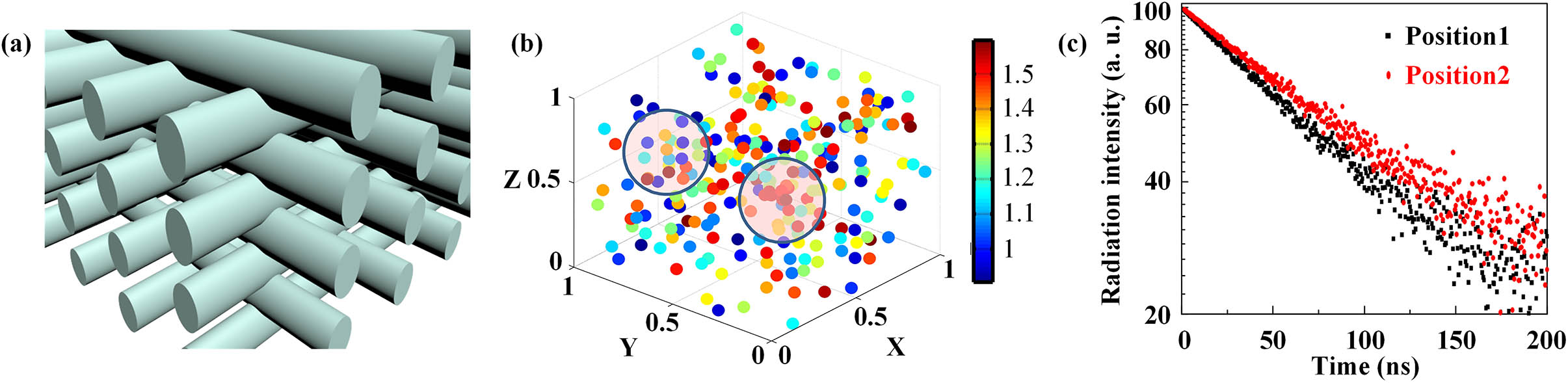
A 3D woodpile PC is shown in Fig. 1(a), and the LDOS in it is position dependent^[12]. Different positions can have significantly different LDOS inside the PC. At some local positions, the SE of an emitter can be suppressed, but at other local positions in the same unit cell of the PC, the SE of the emitter can be enhanced. A typical LDOS map inside a 3D woodpile PC is shown in Fig. 1(b). As LDOS has significant changes within a unit cell of the PC, for a general SE decay lifetime measurement system, when a focal spot is introduced to generate the SE decay signals into a 3D PC, the diffraction-limited excitation focal spot size prevents the achievement of LDOS information of the PC. As a result, only FDOS, which reflects the rough information of the density of states (DOS) within the excitation focal volume, is obtained. The measured FDOS, however, could not reflect the overall SE control ability of the PC. Three reasons can account for this. First, as the confocal detection system is widely adopted to measure the SE control property of a 3D PC as the most powerful tool, this system has a diffraction-limited excitation focal spot size as well as the focal spot size of the detection system. This limits the acquisition of SE decay signals from a required zone inside the unit cell of the PC. Then, SE decay signals from different local positions within the excitation focal spot size contribute differently to the final detected signals due to the local position dependent property of LDOS and the local positional varied excitation light intensities. As a consequence, this FDOS obtained from different volume parts of the unit cell exhibits different SE decay lifetime values. Also, when the SE decay lifetime of assembled emitters in different parts was measured many times, the SE decay lifetime of these emitters exhibited a lifetime distribution rather than a same lifetime value in the real experiment. This happens due to the random property of SE and the error of fitting the measured SE decay curve to get an SE decay lifetime value even if the emitters are exactly the same. Reasonable spatial distribution fluctuation of the emitters also contributes to the lifetime distribution. The lifetime distribution should be broader if the used emitters are not exactly the same. These three reasons make the obtained lifetime value corresponding to the measured FDOS not a representative number for the overall SE control ability of the 3D PC. This also prevents an appropriate comparison of the SE control demonstration for even the same system measured by different people^[13]. For these reasons, the excitation focal spot position averaged FDOS, which corresponds to the FDOS from different volume parts of the unit cell, is proposed to be measured here. Figure 1(c) shows that the SE decay curves obtained at two different local zones are obviously different.

Figure 1.Measurement of SE decay lifetime for embedded emitters in a 3D PC based on a confocal imaging system. (a) A 3D woodpile PC frame diagram. (b) A measurement in a local zone reflects FDOS. (c) Schematic of signals from two local zones gives out different SE decay lifetime values.

A 3D woodpile PC ( $60 μm \times 60 μm \times 10 μm$ in size with a 10 μm thick frame, 24 layers, lattice constant $a = 1150 nm$ , refractive index $n_{r} = 1.52$ ) was first fabricated by two-photon polymerization (2PP) in a photoresin ormocer. PbSe/CdSe core/shell (CS) quantum dots (QDs) were synthesized^[13,14] and attached to the surface of the PC rods as SE decay probes by a molecular linking method^[14]. The fabricated PC with the QD attachment has the $Γ$ -X direction stopgap, which is shown in Fig. 2(a) as a transmission spectrum measured by a Fourier-transform infrared (FTIR) spectroscope. The QDs have emission peak wavelengths matching the $Γ$ -X direction stopgap center wavelength of the PC at 1480 nm [Fig. 2(a)]. To make a comparison, a reference system was designed to be the same QDs attached to the plane surface of a block made of the same material and fabricated by the same conditions as the PC. This reference is designed to rule out any other possible influence on the SE decay lifetime change for QDs inside the PC compared with that in the reference except the influence of the LDOS^[14].

Sign up for Chinese Optics Letters TOC. Get the latest issue of Chinese Optics Letters delivered right to you！Sign up now

Figure 2.(a) Transmission spectra of the woodpile PC in the $Γ$ -X direction before and after the QD attachment and the emission spectrum of the attached QDs with an emission peak wavelength matching the stopgap of the PC in the $Γ$ -X direction. The shadow zone indicates the calculated wavelength range of the $Γ$ -X direction stopgap. (b) Lifetime ratio distribution of 22,300 positions in a unit cell.

A theoretical work was done to investigate the LDOS and FDOS properties of the fabricated PC. The calculation of the LDOS was conducted based on the LDOS theory in a PC^[10] with the plane-wave expansion method^[15–17]. The plane-wave expansion method used to calculate the LDOS in a PC was first developed by X. Wang and B. Gu^[15]. In this method, the electric or magnetic fields are expanded for each field component in terms of the Fourier series components along the reciprocal lattice vector. Each field component corresponds to a plane wave traveling along the reciprocal lattice vector. This method is widely used for solving the band structure of periodic photonic structures. For the specific PC in this work with a woodpile geometry, Liu et al. developed an accurate calculation based on the plane-wave expansion method^[16,17] and made the LDOS calculation for a woodpile PC simple and easy. The calculation formula can be written as $ρ (r, ω) = \sum_{n k} {| E_{n k} (r) |}^{2} δ (ω - ω_{n k}) = \frac{1}{(2 π)^{3}} \sum_{n} \int_{1 B Z} δ (ω - ω_{n k}) {| E_{n k} (r) |}^{2} d^{3} k,$ (1)where $r$ is the local position of an emitter, and $ω$ is the emission frequency of the emitter. ${ω_{n k}, E_{n k} (r)}$ are the radiation field electromagnetic eigen modes in the PC that are mathematically solved by the plane-wave expansion method^[14–16]. The subscript $n$ is the band index. 1BZ is the first Brillouin zone, where the integral of the wave vector $k$ is done. The transition dipole moment of the QDs $d$ is considered as randomly orientated. The parameters of the woodpile PC used in the calculation are as follows: $n_{r} = 1.526$ , $a = 1150 nm$ , elliptical rod short axis $Δ x y = 175 nm$ , and long axis $Δ x z = 350 nm$ . In a unit cell, 22,300 local positions outside the PC rods were calculated. The calculation is done with a home-developed computer program, and a single lattice is used to dot the simulation. To be consistent with the experiment, local positions with minimum distance to the PC rods within the experimental allowed range were selected. As four layers of QDs were attached to the surface of the PC rods and the QDs had an average size of 5 nm, a distance range of 0–20 nm was used. The SE decay rate of an emitter in the PC, which is the reciprocal of its SE decay lifetime, is proportional to the corresponding LDOS^[10]. That is, $Γ (r, ω) = ρ (r, ω) d^{2} ω / (6 ℏ ε_{0}) = 1 / τ,$ (2)where $ℏ$ is the reduced Planck constant, and $ε_{0}$ is the vacuum permittivity. So, the SE decay lifetime of the QDs at the 22,300 local positions inside the PC can be calculated as a ratio to that of the QDs in the reference. The lifetime ratio distribution was plotted in Fig. 2(b). From this data, the SE of the QDs inside the PC is suppressed with an average of 19.9% longer lifetime. This is because the SE of the QDs is tuned by the photonic stopgap of the PC. When the emission wavelength of the QDs lies in the wavelength range of the PC stopgap, which corresponds to decreased LDOS, the SE is suppressed. The SE at some particular position is suppressed with a 60% longer lifetime. Compared with this, the SE at some other particular positions is enhanced with a 10% shorter lifetime.

It is clearly evident that the SE decay lifetime of the QDs inside the PC shows a significant fluctuation in Fig. 2(b). In the SE decay lifetime experiment, when a focal spot with the size about half the size of the unit cell was used to excite the SE of the QDs inside the PC, as only the QDs inside the focal spot size were excited, a SE decay lifetime corresponding to the FDOS was obtained. For QDs, they are artificial atoms synthesized by a wet chemical method^[18,19]. It is inevitable that these QDs are not exactly the same. For example, the size of the QDs has a distribution. Even a selective precipitation method was adopted to get uniform sized QDs as much as possible; a 5% size variation is still reasonable^[18,19]. As QDs have the essential advantages^[20,21] for SE decay lifetime measurement in this work, such as moderate lifetime value, quasi-two-level system, excellent anti-photobleaching property, and high emission quantum efficiency, they were used as the SE probes as well as we could. This can contribute to a broader lifetime distribution than that if the emitters were exactly the same, which is quite challenging in the experiment.

As the QDs inside the PC have an intrinsic lifetime distribution, it is important to have a study about the FDOS if the same lifetime measurements were done many times at different excitation focal spot relative positions to a unit cell of the PC. This can give out a distribution of the obtained FDOS. Consider a simplified model, which does not include the SE decay signal contribution difference of the QDs inside the excitation focal spot; if the SE decay lifetime experiment is done at random excitation focal spot relative positions, the average SE decay lifetime value can be simulated. A typical curve about the simulated average lifetime value ratio to the average value of the 22,300 positions versus the SE decay lifetime measurement times was plotted in Fig. 3(a). When the measurement times become less, as the measured lifetime has the random property from the random selection of the excitation focal spot relative positions, the average lifetime exhibits a significant difference from the overall average value. This difference becomes narrower when more times of measurements are conducted. Figures 3(b) and 3(c) show 10,000 times of the simulation for two time measurements and 100 time measurements with random positions. It is clearly shown that the average lifetime value corresponding to the position averaged FDOS with sufficient measurement times can reflect the overall average value of LODS with small randomly induced error. In Fig. 3(d), the more the measurement times, the less the error. When 120 times of measurement are conducted, the average lifetime value corresponding to the position averaged FDOS can reflect the overall average value of the LDOS with less than 1% error within a 95% confidence interval.

Figure 3.Simulation of random excitation focal spot position averaged lifetime value ratio to the overall averaged lifetime value with different measurement times. (a) A typical average lifetime value ratio change with measurement times. (b) Lifetime ratio distribution of 2 measurement times for 10,000 times simulation. (c) Lifetime ratio distribution of 100 measurement times for 10,000 times simulation. (d) Confident up and down limits corresponding to 95% confident level vary with the measurement times with random excitation focal spot positions.

The experimental measurement of SE decay lifetime of the QDs inside the PC compared with that in the reference was done. The SE decay lifetime of the QDs was measured by a time-correlated single-photon counting system, which is in conjunction with a home-made confocal detection system with a high numerical aperture ( $NA = 0.8$ ) objective^[14]. The excitation laser beam was operated at the wavelength of 1064 nm with a repetition rate of 5 MHz and pulse duration of 49 ps. The excitation focal spot volume is smaller than that of the unit cell of the PC. The excitation laser intensity was kept as low as possible to avoid fast Aüger recombination. Typical decay curves of the QDs inside the PC and in the reference are shown in Fig. 4(a). The single exponential decay function was used to fit the SE decay curve to get the SE decay lifetime value. As the PC fabricated in this work has a finite size of $60 μm \times 60 μm \times 10 μm$ , the finite size induced surface defect can influence the SE suppression effect of the PC. Because the LDOS calculation was done based on a PC with an infinite size, the SE decay lifetime measurement was conducted at the geometric center of the PC (around the position of 30 μm–30 μm–5 μm X–Y–Z) with $\pm 3.5 μm - 3.5 μm - 1 μm$ tolerance to be consistent with the calculation.

Figure 4.(a) Typical measured decay curves that are fitted with single exponential decay function for QDs in the PC and in the reference. (b) Distribution of the SE decay lifetime value for QDs inside the PC and in the reference.

SE decay curves from 128 random relative positions of the excitation focal spot in the PC were measured. SE decay curves from 121 random positions of the excitation focal spot in the reference were also measured with the same conditions as those in the PC as a comparison. The lifetime value distributions of them are shown in Fig. 4(b). As was expected, the lifetime value of the QDs in the reference has a distribution. Compared with this, the lifetime distribution of the QDs inside the PC is broader with a longer shift. The broader distribution can be attributed to the LDOS fluctuation inside the PC. The relatively broader value (the relative full width at half-maximum of the lifetime distribution divided by the average lifetime value) is 3.2%. The longer lifetime distribution shift comes from the photonic stopgap effect of the PC. The averaged lifetime value of the QDs inside the PC is 20.5% longer than that of the reference, which is consistent with the theory value of 19.9%. This lifetime distribution of the QDs inside the PC compared with that of the reference reflects the overall SE control ability of the PC with local positional details lost. As the local positions with 60% longer SE decay lifetime and 10% shorter SE decay lifetime only occupy less than 1% of the total positions inside the unit cell, this information is totally lost in the measured lifetime distribution. A higher spatial resolution measurement can get a lifetime distribution with details more similar to the calculated one. However, the 20.5% longer average lifetime and 3.2% broader lifetime distribution can be used as accurate characteristic parameters to indicate the overall SE control ability of the PC.

To conclude, accurately measuring the overall SE control ability of a 3D PC encounters the problem of FDOS. The measuring of the position averaged FDOS has been theoretically and experimentally investigated in this work, which confirms that position averaged FDOS rather than only the FDOS can accurately reflect the overall SE control ability of a PC with two characteristic parameters. Our work contributes to the comprehensive characterizing of the SE control performance of photonic devices for real application with quantified parameters.

References

[1] Z. Wang, K. Su, B. Feng, T. Zhang, W. Huang, W. Cai, W. Xiao, H. Liu, J. Liu. Chin. Opt. Lett., 16, 011301(2018).

[2] B. Ma, K. Kafka, E. Chowdhury. Chin. Opt. Lett., 15, 051901(2017).

[3] K. Receveur, K. Wei, M. Hadjloum, M. El Gibari, A. De Rossi, H. W. Li, A. S. Daryoush. Chin. Opt. Lett., 15, 010003(2017).

[4] S. Noda, K. Tomoda, N. Yamamoto, A. Chutinan. Science, 289, 604(2000).

[5] M. D. Leistikow, A. P. Mosk, E. Yeganegi, S. R. Huisman, A. Lagendijk, W. L. Vos. Phys. Rev. Lett., 107, 193903(2011).

[6] Z. Lin, A. Pick, M. Lončar, A. W. Rodriguez. Phys. Rev. Lett., 117, 107402(2016).

[7] M. Pelton. Nat. Photon., 9, 427(2015).

[8] X.-H. Wang, R. Wang, B.-Y. Gu, G.-Z. Yang. Phys. Rev. Lett., 88, 19(2002).

[9] X.-H. Wang, B.-Y. Gu, R. Wang, H.-Q. Xu. Phys. Rev. Lett., 91, 11(2003).

[10] M. J. Ventura, M. Gu. Adv. Mater., 20, 1329(2008).

[11] F. A. Inam, T. Gaebel, C. Bradac, L. Stewart, M. J. Withford, J. M. Dawes, J. R. Rabeau, M. J. Steel. New J. Phys., 13, 073012(2011).