Author Affiliations
1Key Laboratory of Optoelectronic Information Technology Ministry of Education, School of Precision Instrument & Opto-electronics Engineering, Tianjin University, Tianjin 300072, China2Lepu Medical Technology (Beijing) Co., Ltd., Beijing 102200, China3Southwestern Lu Hospital, Liaocheng, Shandong 252325, Chinashow less
Fig. 1. Ideal hypothesis diagrams. (a) The mask image that meets the ideal hypothesis; (b) The situation that does not meet the ideal hypothesis
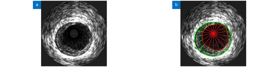
Fig. 2. Modeling schematics. (a) Original image of IVUS; (b) Schematic diagram of modeling result. The intima contour and media contour are marked with red and green curves, respectively. The modeling results of the lumen area and plaque area are marked with red and green line segments, respectively
Fig. 3. The proposed dense distance of regression network
Fig. 4. Schematic diagram of the intersection of the true value and the predicted value patch area. Note: For the convenience of observation, the true value ray and the predicted value ray are staggered by a certain angle, and the two are actually on the same ray
Fig. 5. The graph of JM changing with the number of rays
Fig. 6. Visualization of segmentation results of different modeling methods
Fig. 7. Comparison of the visual effects of the segmentation results
Fig. 8. Linear regression analysis of key clinical parameters
Fig. 9. Bland-Altman analysis of key clinical parameters
Table 1. Information of the IVUS dataset
Backbone | SEB num | JM | | HD/mm | | PAD | | TER | Med | Lum | Plaque | Med | Lum | Med | Lum | - | ResNet18 | 0 | 0.8630 | 0.8589 | 0.6935 | | 0.2361 | 0.1501 | | 0.1077 | 0.1038 | | 0 | 1 | 0.8658 | 0.8520 | 0.6947 | 0.2252 | 0.1603 | 0.1048 | 0.1174 | 0 | 2 | 0.8659 | 0.8634 | 0.6979 | 0.2167 | 0.1555 | 0.1078 | 0.1039 | 0 | 3 | 0.8655 | 0.8598 | 0.7016 | 0.2258 | 0.1513 | 0.1117 | 0.1038 | 0 | ResNet34 | 0 | 0.8866 | 0.8674 | 0.7302 | | 0.1906 | 0.1446 | | 0.0849 | 0.0950 | | 0 | 1 | 0.8803 | 0.8606 | 0.7173 | 0.2080 | 0.1475 | 0.0891 | 0.1013 | 0 | 2 | 0.8716 | 0.8610 | 0.7071 | 0.2357 | 0.1558 | 0.0979 | 0.1046 | 0 | 3 | 0.8818 | 0.8574 | 0.7167 | 0.2227 | 0.1559 | 0.0833 | 0.1077 | 0 | ResNet50 | 0 | 0.8804 | 0.8692 | 0.7221 | | 0.1855 | 0.1462 | | 0.0937 | 0.0967 | | 0 | 1 | 0.8738 | 0.8687 | 0.7131 | 0.2248 | 0.1385 | 0.0978 | 0.0946 | 0 | 2 | 0.8760 | 0.8671 | 0.7152 | 0.2266 | 0.1445 | 0.0901 | 0.0990 | 0 | 3 | 0.8805 | 0.8757 | 0.7211 | 0.2153 | 0.1351 | 0.0915 | 0.0879 | 0 | ResNet101 | 0 | 0.8853 | 0.8665 | 0.7298 | | 0.2014 | 0.1380 | | 0.0860 | 0.0928 | | 0 | 1 | 0.8910 | 0.8646 | 0.7346 | 0.1873 | 0.1553 | 0.0816 | 0.1099 | 0 | 2 | 0.8934 | 0.8738 | 0.7430 | 0.1761 | 0.1355 | 0.0794 | 0.1005 | 0 | 3 | 0.8902 | 0.8725 | 0.7337 | 0.1775 | 0.1396 | 0.0745 | 0.0827 | 0 | ResNet152 | 0 | 0.8852 | 0.8646 | 0.7302 | | 0.2012 | 0.1412 | | 0.0881 | 0.1036 | | 0 | 1 | 0.8845 | 0.8711 | 0.7256 | 0.2073 | 0.1402 | 0.0874 | 0.0958 | 0 | 2 | 0.8974 | 0.8708 | 0.7424 | 0.1879 | 0.1481 | 0.0736 | 0.0962 | 0 | 3 | 0.8849 | 0.8627 | 0.7255 | 0.2101 | 0.1545 | 0.0854 | 0.1088 | 0 |
|
Table 2. The performance of the proposed method under different depths of backbone and different numbers of SEB modules
Loss function | JM | | HD/mm | | PAD | | TER | Med | Lum | Plaque | Med | Lum | Med | Lum | - | Smoothl1 | 0.8732 | 0.8698 | 0.7047 | | 0.2131 | 0.1436 | | 0.0999 | 0.0930 | | 0 | Ll+Lp | 0.8850 | 0.8757 | 0.7319 | 0.2145 | 0.1350 | 0.0912 | 0.0929 | 0 | Lm+Lp | 0.8904 | 0.8636 | 0.7313 | 0.1997 | 0.1509 | 0.0794 | 0.1116 | 0 | Ll+Lm | 0.8808 | 0.8736 | 0.7183 | 0.2172 | 0.1447 | 0.0894 | 0.0892 | 0 | IVUS Polar IoU Loss | 0.8934 | 0.8738 | 0.7430 | 0.1761 | 0.1355 | 0.0794 | 0.1005 | 0 |
|
Table 3. Experimental results with different loss functions
建模方式 | Loss | JM | | HD/mm | | PAD | | TER | Med | Lum | Plaque | Med | Lum | Med | Lum | - | Ellipse | Smoothl1 | 0.8208 | 0.8124 | 0.6100 | | 0.2633 | 0.1793 | | 0.1399 | 0.1402 | | 0.0767 | PCM-PK | 0.8732 | 0.8698 | 0.7047 | 0.2131 | 0.1436 | 0.0999 | 0.0930 | 0 |
|
Table 4. Experimental results with different modeling methods
| Backbone | JM | | HD/mm | | PAD | | TER | Med | Lum | Plaque | Med | Lum | Med | Lum | - | SegNet[30] | - | 0.8856 | 0.8618 | 0.7148 | | 0.5367 | 1.5783 | | 0.0948 | 0.1245 | | 0.2328 | UNet[31] | - | 0.8857 | 0.8846 | 0.7300 | 0.4700 | 0.1776 | 0.0956 | 0.0950 | 0.1319 | Deeplabv3+[29] | ResNet101 | 0.9026 | 0.8886 | 0.7567 | 0.2427 | 0.1302 | 0.0677 | 0.0787 | 0.0390 | Ours | ResNet101 | 0.8934 | 0.8738 | 0.7430 | 0.1761 | 0.1355 | 0.0794 | 0.1005 | 0 |
|
Table 5. Performance comparison of different segmentation models
| 斜率 | 截距 | Pearson相关系数 | LCSA | 0.9825 | 0.2359 | 0.9427 | VCSA | 1.1259 | −1.3911 | 0.9626 | PCSA | 1.2016 | −1.5044 | 0.9432 |
|
Table 6. Results of linear regression analysis of key clinical parameters
| 均值 | 均值偏移 | 偏移程度/% | 离群值比例/% | LCSA | 5.9898 | −0.1320 | −2.20 | 5.25 | VCSA | 15.8044 | −0.5628 | −3.56 | 6.59 | PCSA | 9.8146 | −0.4308 | −4.40 | 7.27 |
|
Table 7. Results of Bland-Altman analysis of key clinical parameters