
Tao Wang, Zhan Li, Sheng Wang, Weilin Qiao, Jun Wu. Blades Model Reconstruction Based on Speckle Vision Measurement[J]. Laser & Optoelectronics Progress, 2019, 56(1): 011501
- Laser & Optoelectronics Progress
- Vol. 56, Issue 1, 011501 (2019)
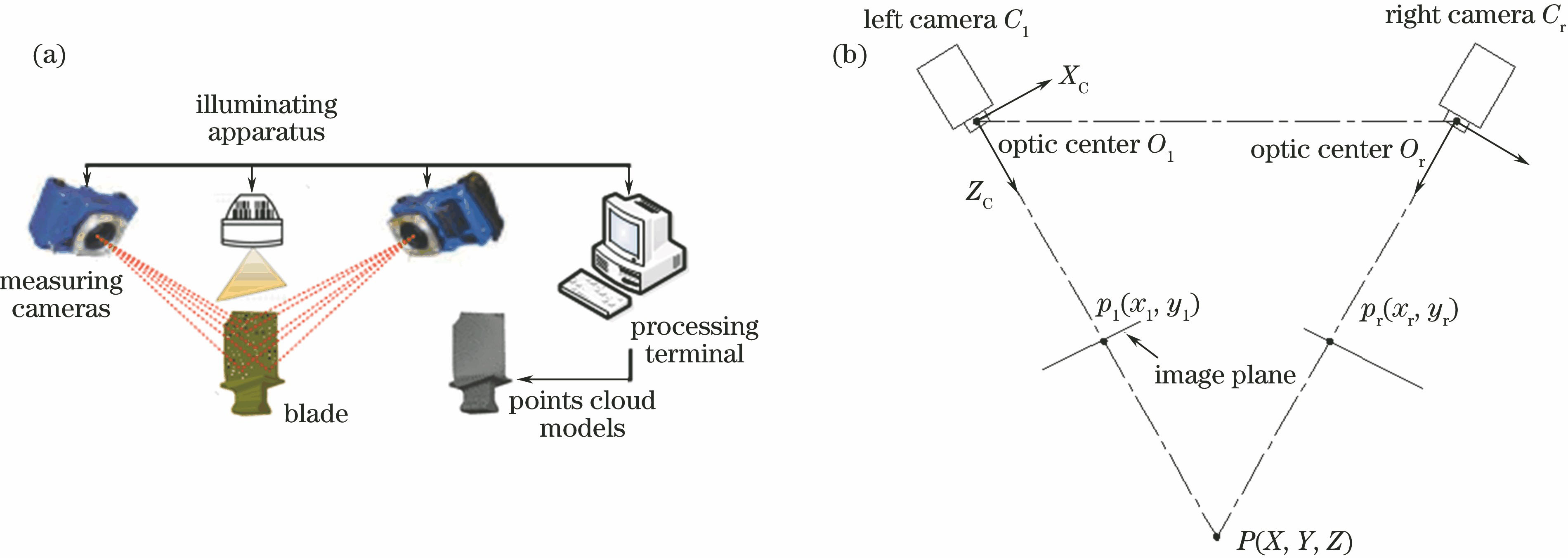
Fig. 1. (a) Speckle vision system and (b) its two-dimensional schematic diagram
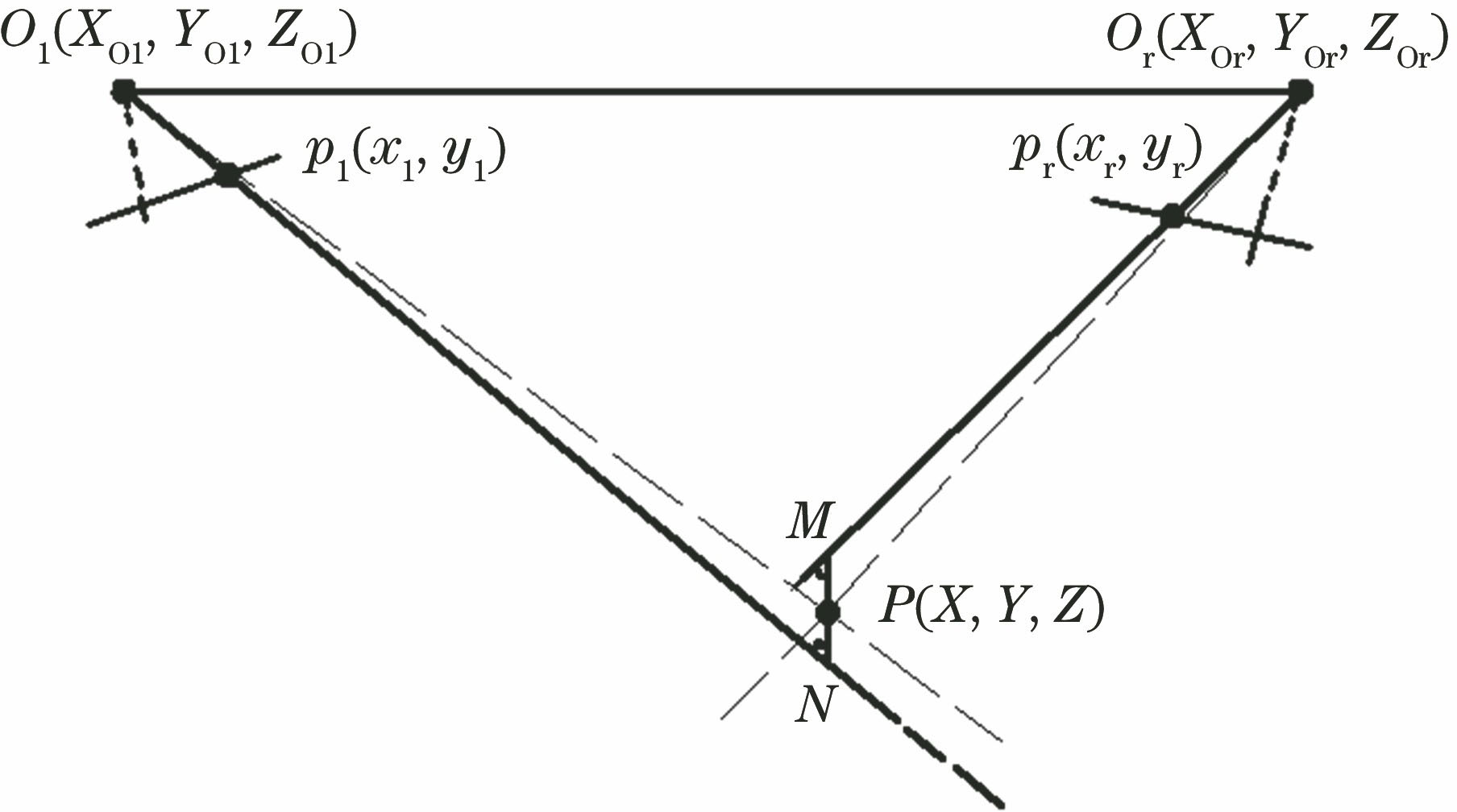
Fig. 2. Diagram of spatial intersection
Fig. 3. Schematic of splicing principle
Fig. 4. Flow chart of boundary point extraction
Fig. 5. (a) Actual measuring platform and (b) calibration target
Fig. 6. Binocular camera internal parameter calibration residuals. (a) Left camera; (b) right camera
Fig. 7. Stereo matching of speckles. (a) Images to be matched; (b) matching images
Fig. 8. Blade point cloud reconstruction. (a) Front blade point cloud; (b) rear blade point cloud
Fig. 9. Image processing of some markers
Fig. 10. Visual splicing of blade surface point cloud
Fig. 11. (a) Boundary points of front blade; (b) fitting curve with the cubic B-spline method
Fig. 12. Splicing of blade point cloud fitting
Fig. 13. (a) Fitting surface of front blade point cloud; (b) fitting surface of rear blade point cloud; (c) overall surface configuration of the blade
|
Table 1. Calibration results of measuring system external parameters
|
Table 2. Point cloud fitting analysis
|
Table 3. Geometrical parameter errors of blade surface

Set citation alerts for the article
Please enter your email address
© Copyright 2018-2021 | Chinese Laser Press. All Rights Reserved 沪ICP备15018463号-20