
Ying Han, Jing Yuan, Jiangsheng Si, Dehe Yang. Real-Time Detection of Small Obstacles Based on 16-Ray Lidar Point Cloud[J]. Laser & Optoelectronics Progress, 2021, 58(12): 1228001
- Laser & Optoelectronics Progress
- Vol. 58, Issue 12, 1228001 (2021)
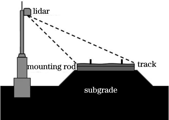
Fig. 1. Scenery for railway detection
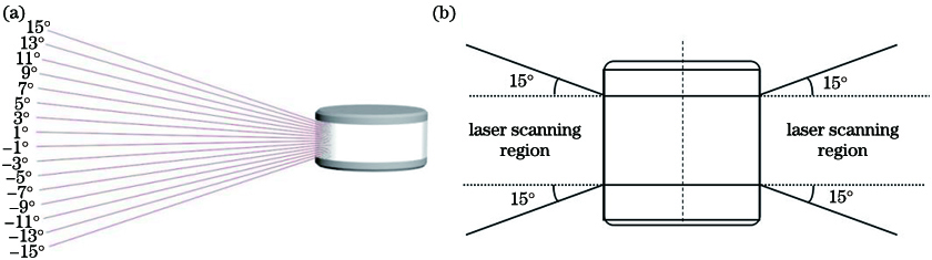
Fig. 2. Schematic of R-Fans-16 lidar.(a) Lidar model; (b) scanning angle
Fig. 3. R-Fans-16 coordinate system and schematic of parameters. (a) R-Fans-16 coordinate system;(b) schematic of angles
Fig. 4. Scanning point cloud map of scene
Fig. 5. Lidar fixed on angular displacement platform. (a) Angular displacement platform; (b) coordinate center of angular displacement platform; (c) platform and lidar
Fig. 6. Point cloud map of angular displacement platform rotated by 2°
Fig. 7. Scenery for lidar monitoring railway. (a) Front view; (b) left view; (c) top view
Fig. 8. Radar system with triangular base. (a) Perspective view; (b) front view; (c) left view; (d) top view
Fig. 9. Schematic of lidar rotation and coordinate transformation system. (a) Radar with added angular displacement platform; (b) lidar self-rotation and simultaneous rotation with angular system displacement platform; (c) coordinate transformation system
Fig. 10. Angle change during lidar scanning process. (a) Simulation of lidar scanning scene; (b) relationship between lidar self-rotation and lidar rotaion driven by angular displacement platform
Fig. 11. Point cloud map of angular displacement platform rotated by 14°
Fig. 12. Effects after deletion of duplicate data by different methods. (a) Direct deletion method; (b) mean method
Fig. 13. Flow chart of obstacle detection
Fig. 14. Pass-through filtering result
Fig. 15. 3D region segmentation based on octree voxelization . (a) 3D representation of space;(b) octree hierarchical structure
Fig. 16. Schematic of point cloud difference treatment. (a) Background point cloud; (b) point cloud for real-time detection; (c) result after difference treatment
Fig. 17. Statistical filtering results under different conditions.(a) k=20,ε1=1; (b) k=5,ε1=0.1; (c) k=20,ε1=0.1
Fig. 18. Lidar measurement objects and point cloud map. (a) 3D lidar measurement scene; (b) point cloud map; (c) practical obstacle images
Fig. 19. Resutls of obstacle detection based on 16-ray point cloud. (a) Point cloud of real-time detection on right of lidar; (b) result after pass-through filtering; (c) result after difference treatment; (d) result after denoising;(e) marking result of obstacle on right; (f) marking result of obstacle on left
Fig. 20. Results of obstacle detection based on 1-ray point cloud. (a) Result after pass-through filtering; (b) result after difference treatment; (c) result after denoising; (d) marking result of obstacle on left; (f) marking result of obstacle on right
Fig. 21. 16-ray point cloud for real-time detection of obstacle
Fig. 22. Comparison between 1-ray point cloud and 16-ray point cloud. (a) 1-line point cloud; (b) 16-line point cloud

Set citation alerts for the article
Please enter your email address
© Copyright 2018-2021 | Chinese Laser Press. All Rights Reserved 沪ICP备15018463号-20