
Lemeng Leng, Zhaobang Zeng, Guihan Wu, Zhongzhi Lin, Xiang Ji, Zhiyuan Shi, Wei Jiang. Phase calibration for integrated optical phased arrays using artificial neural network with resolved phase ambiguity[J]. Photonics Research, 2022, 10(2): 347
- Photonics Research
- Vol. 10, Issue 2, 347 (2022)
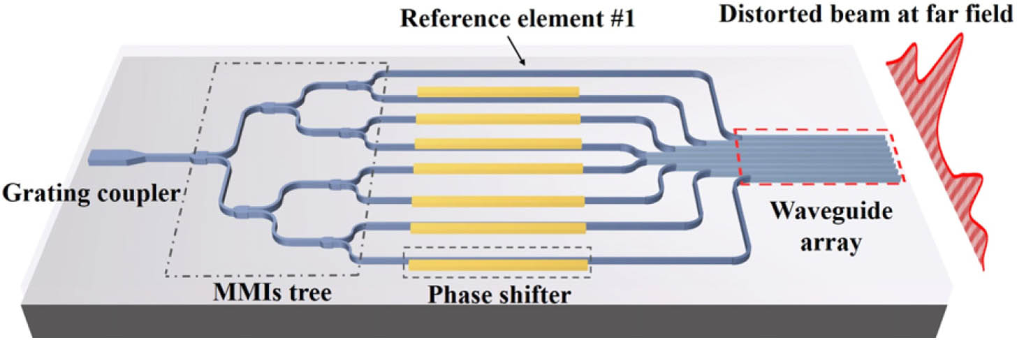
Fig. 1. Schematic view of an integrated OPA, along with the far-field pattern.
![Example of the far-field patterns for feeding the neural network, I(φ,θ) and I(φ+ϕ,θ), generated by the OPA with (a) phase error of φ and (b) additional phase mask of ϕ. (c)–(f) Build ANNs with different architectures. The green and purple arrows indicate the backpropagation of the ANNs using a loss function of MSE or CMSE. The red arrows indicate the configurations of the data for input [using pattern 1, I(φ,θ), with Nθ data points or the combination of pattern 1 and pattern 2, I(φ,θ),I(φ+ϕ,θ), with 2Nθ data points].](/richHtml/prj/2022/10/2/02000347/img_002.jpg)
Fig. 2. Example of the far-field patterns for feeding the neural network, I ( φ , θ ) I ( φ + ϕ , θ ) φ ϕ I ( φ , θ ) N θ I ( φ , θ ) , I ( φ + ϕ , θ ) 2 N θ
Fig. 3. Loss of (a) Net 1, (b) Net 2, (c) Net 3, and (d) Net 4 with the architecture in Figs. 2 (c)–2 (f) evolving with training epochs. Red curves indicate loss of the training set, and blue curves indicate loss of the validation set.
Fig. 4. Simulated performance of the ANNs using four randomly selected samples i) to iv) in testing set. Each sample is signified with a different color. (a1)–(a4) Far-field profiles before calibration. Beam profiles after calibration from the output of (b1)–(b4) Net 1; (c1)–(c4) Net 2; (d1)–(d4) Net 3; and (e1)–(e4) Net 4. The sidelobe levels of the formed beams are noted in (d1)–(d4) and (e1)–(e4). All figures share the same axis.
Fig. 5. Schematic of the experimental setup for automatic calibration via Net 4 (FPC, fiber polarization controller; SMF, single-mode fiber).
Fig. 6. Calibration for two arbitrarily selected devices i) and ii); experimentally measured far-field pattern before calibration (blue line) and calculated far-field pattern (red line) using the ANN-predicted phase error for (a) device i) and (d) device ii); measured beam profile after calibration using ANN for (b) device i) and (e) device ii); condensed beam profile after calibration using PSO for (c) device i) and (f) device ii).
Fig. 7. (a) Measured resistances of the phase shifters in our 16-channel OPA; (b) measured (scatter) and fitted (line) heating power versus output intensity for the phase shifter embedded in an interferometer.
Fig. 8. Distribution of calculated S
Fig. 9. Accuracy of the ANN versus α β γ
Fig. 10. Simulated PSO-based calibration statistics for 500 OPA devices, compared with ANN-model test results. (a) Simulated accuracy of the test set using PSO algorithms with different swarm sizes (the accuracy of ANN is marked for comparison); (b) simulated sidelobe suppression ratio statistics (the average and very small standard deviation of ANN are marked by a red line and a narrow shaded stripe, respectively); (c) total number of experimental evaluations (equivalent to the number of far-field measurements) required for this iterative method for 500 OPA devices. Note that the y
Fig. 11. Measured 2D beam profiles (a) before calibration, (b) after calibration using ANN, and (c) after calibration using PSO for device i) in Fig. 6 .

Set citation alerts for the article
Please enter your email address
© Copyright 2018-2021 | Chinese Laser Press. All Rights Reserved 沪ICP备15018463号-20