
J. J. Pilgram, M. B. P. Adams, C. G. Constantin, P. V. Heuer, S. Ghazaryan, M. Kaloyan, R. S. Dorst, D. B. Schaeffer, P. Tzeferacos, C. Niemann. High repetition rate exploration of the Biermann battery effect in laser produced plasmas over large spatial regions[J]. High Power Laser Science and Engineering, 2022, 10(2): 02000e13
- High Power Laser Science and Engineering
- Vol. 10, Issue 2, 02000e13 (2022)
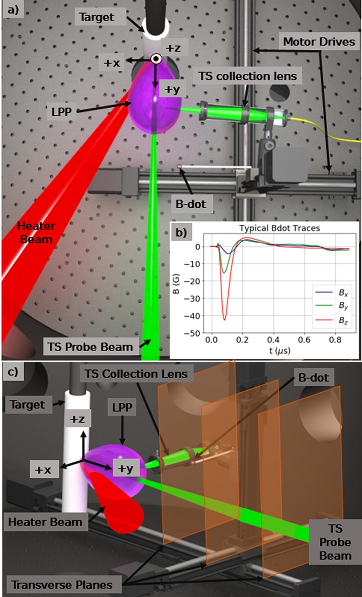
Fig. 1. A rendering of the experimental setup. (a) Top view. The origin of the coordinate system is the laser spot on target, with the corresponding axis directions as depicted. (b) Typical B-dot probe traces for all three axes of the probe. (c) Side view. The translucent orange rectangles represent the planes in which magnetic field data were collected.
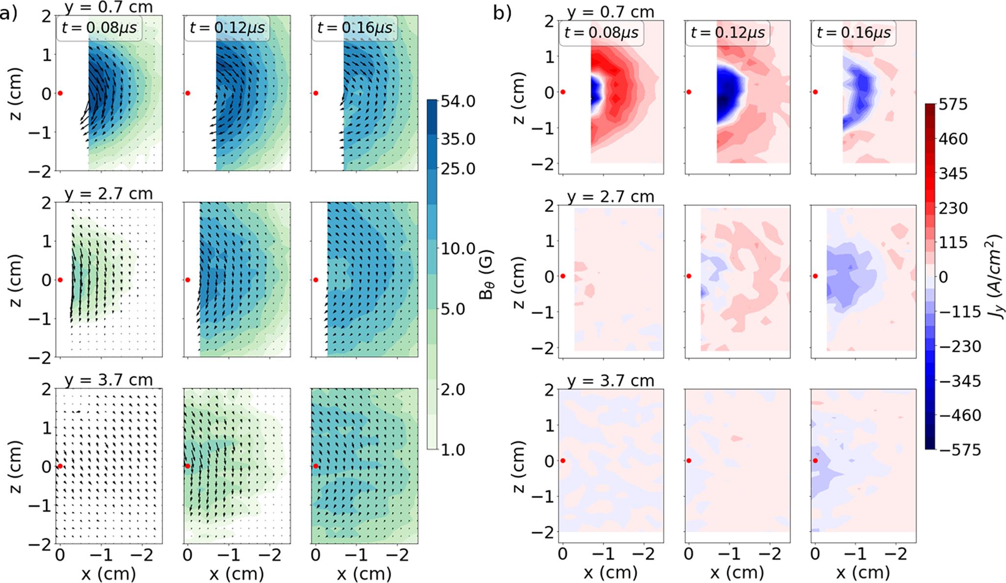
Fig. 2. ( a) Contour plots of azimuthal magnetic field structure in several transverse planes at three representative times. Magnetic field vectors are denoted by the black arrows. (b) The calculated current density along the plasma blow-off axis in several transverse planes at three representative times. The red dot represents the laser spot and white spaces are positions that the probe could not reach due to mechanical constraints.
Fig. 3. Plot of maximum azimuthal magnetic field versus distance from the laser spot. The times at which each point occurs correspond to the times in Figure 5 . A  curve (red line) agrees well with the data with a value of
  .
.
curve (red line) agrees well with the data with a value of . Fig. 4. A streak plot of the total magnetic field (contour) from a  -lineout at
  mm,
mm,  mm. Linear fits (orange lines) are applied to features of the magnetic field streak plot to determine the speed of different magnetic field features.
-lineout at mm, mm. Linear fits (orange lines) are applied to features of the magnetic field streak plot to determine the speed of different magnetic field features. Fig. 5. Plot of the maximum of the azimuthal magnetic field observed on the magnetic flux probe (black) at different planes as a function of time. A linear fit (blue line) to the data indicates a speed of 330 km s−1.
Fig. 6. (a) Visualization of the 2D simulation domain for the  plane, that is,
  , at
, at  for the laser-facing side of the target. The black semi-circle region denotes the rod that supports the target material (grey). The Peening laser beam enters the simulation domain at a 34° angle from the
  -direction for positive values of
  , reflecting the geometry of the experimental setup provided in
 Figure 1 (a). The region visualized in the provided simulation results (Figures 7 and 8 ) is enclosed by the dashed red line. (b) The power profile used to model the Peening laser heater beam in FLASH with a peak of  W at 7.5 ns, which allows 10 J of energy to be deposited to the target over 15 ns as in the experiment.
plane, that is, , at for the laser-facing side of the target. The black semi-circle region denotes the rod that supports the target material (grey). The Peening laser beam enters the simulation domain at a 34° angle from the -direction for positive values of , reflecting the geometry of the experimental setup provided in W at 7.5 ns, which allows 10 J of energy to be deposited to the target over 15 ns as in the experiment. Fig. 7. Visualization of the FBB 2D FLASH simulation for (a) the electron number density  , (b) the electron temperature
  , (c) the magnitude of the velocity and (d) the magnetic Reynolds number at 150 ns after the laser fires. We describe the threshold applied to these visualizations in the text.
, (b) the electron temperature , (c) the magnitude of the velocity and (d) the magnetic Reynolds number at 150 ns after the laser fires. We describe the threshold applied to these visualizations in the text. Fig. 8. A visualization of the magnetic field values within the LPP region 150 ns after laser fires. (a) Results from a simulation where the Biermann battery source term was calculated only during the 15 ns duration of the laser (LOBB case) and (b) results where the Biermann battery source term was calculated for the entire simulation duration of 400 ns (FBB case). Provided in (c) are line-outs from (a) LOBB and (b) FBB simulations taken at  cm and
  cm away from the target.
cm and cm away from the target. 
Set citation alerts for the article
Please enter your email address
© Copyright 2018-2021 | Chinese Laser Press. All Rights Reserved 沪ICP备15018463号-20