
J. J. Pilgram, M. B. P. Adams, C. G. Constantin, P. V. Heuer, S. Ghazaryan, M. Kaloyan, R. S. Dorst, D. B. Schaeffer, P. Tzeferacos, C. Niemann, "High repetition rate exploration of the Biermann battery effect in laser produced plasmas over large spatial regions," High Power Laser Sci. Eng. 10, 02000e13 (2022)
- High Power Laser Science and Engineering
- Vol. 10, Issue 2, 02000e13 (2022)
Abstract
1 Introduction
Magnetic fields are prevalent throughout the universe. The generation of cosmic magnetism represents an important problem in modern astrophysics. As described by Kulsrud and Zweibel[1], the cosmological evolution of the universe cannot be fully understood without solid knowledge of the origin of magnetic fields, structures and evolution. These fields are hard to detect as they are very weak (in the micro-Gauss range) and far away[1–4]. Diagnostic techniques, such as Faraday rotation and Zeeman splitting, are difficult to implement in such contexts[1,5,6]. However, laboratory astrophysics experiments, which reproduce astrophysical plasmas scaled by dimensionless parameters, can supplement observational measurements by addressing these limitations[7,8]. Thus, the marriage of astrophysical observation and theory, laboratory experimentation using laser-produced plasmas (LPPs) and computational modeling of such scenarios aid in the pursuit of answering questions on cosmic magnetic field generation.
One predominant theory for primordial cosmic magnetic seed fields is the Biermann battery mechanism[1,9–11], which is a thermo-electric process that spontaneously generates magnetic fields in plasmas via non-parallel temperature and density gradients. This effect was first described by Ludwig Biermann in 1949[12] and has been studied in a variety of plasma experiments[13–18] due to its importance not only for cosmic fields but also for its influential role in many laboratory plasma phenomena, such as magnetic reconnection[19], laboratory shocks[11,20] and components of inertial confinement fusion schemes[21,22].
LPP platforms are commonly used to study these spontaneously generated magnetic fields[18,23]. Not only do LPPs naturally produce the density and temperature gradients needed to precipitate the Biermann battery, but also the magnetic fields generated in laser experiments by the Biermann battery mechanism play a significant role in the energy transport in plasmas, affecting particle dynamics[24], leading to hot spots[25], fast electrons and ions[26], and producing large magnetic pressures (i.e., high plasma-
Sign up for High Power Laser Science and Engineering TOC. Get the latest issue of High Power Laser Science and Engineering delivered right to you!Sign up now
The amplitudes of laboratory-generated Biermann fields range from weak (a few micro-Gauss) to very strong (mega-Gauss)[27,28] and have shown a direct dependence on the laser irradiation intensity in the range of 1012–1014 W/cm2. McLean et al.[29] detected up to 300 kG fields; Stamper et al. demonstrated MG fields at 1015 W/cm2, as did Pisarczyk et al.[14] and Gopal et al.[15] in plasmas generated by lasers with intensities above 1016 W/cm2. In all cases, the peak amplitudes were found very close to the target surfaces, at distances of less than 1 cm. A 2D map of the Biermann battery effect was generated by McKee et al.[16] extending 2 cm from the target surface. These measurements also confirmed the findings of Bird et al.[30] that stronger fields may be generated in the presence of a background gas.
Although this large body of work establishes a foundation for understanding the process of magnetic field formation, there is a lack of data on how Biermann fields behave at larger spatial scales, including the range over which magnetic advection or diffusion dominates. In this paper we present a new high repetition rate (HRR) experimental platform for studying the generation and evolution of Biermann magnetic fields in LPPs over large (tens of cm) spatial scales. By combining an HRR laser driver and motorized magnetic flux probe, we obtain over thousands of shots high spatial resolution, 3D maps of the evolution of Biermann-generated magnetic fields and current density structures. Additional HRR measurements with an optical Thomson scattering probe beam allow us to measure plasma density and temperature. From this data we directly calculate the magnetic Reynolds number and show that magnetic advection dominates at distances more than or equal to
2 Theoretical background
The evolution of the magnetic fields in a non-ideal resistive magnetohydrodynamics framework is described by an induction equation of the following form:
where
In LPPs, the primary temperature gradient is perpendicular to the axis of the plasma plume and the primary density gradient is normal to the target surface (with higher density closer to the target). The electrons collectively move parallel with the pressure gradient at higher velocities than the heavier ions. This action generates an electromotive force (EMF). By Faraday’s law, this EMF in turn creates a magnetic flux, and thus a magnetic field is spontaneously created in an azimuthal direction around the plasma blow-off axis. The term in the induction equation that is of interest in this study is the source term:
where
To determine if diffusion of the magnetic field dominates over advection in our plasma, we estimate the magnetic Reynolds number. The magnetic Reynolds number is found by non-dimensionalizing Equation (1). This number is a dimensionless ratio between the magnetic advection and diffusion within a plasma and is defined as follows:
where
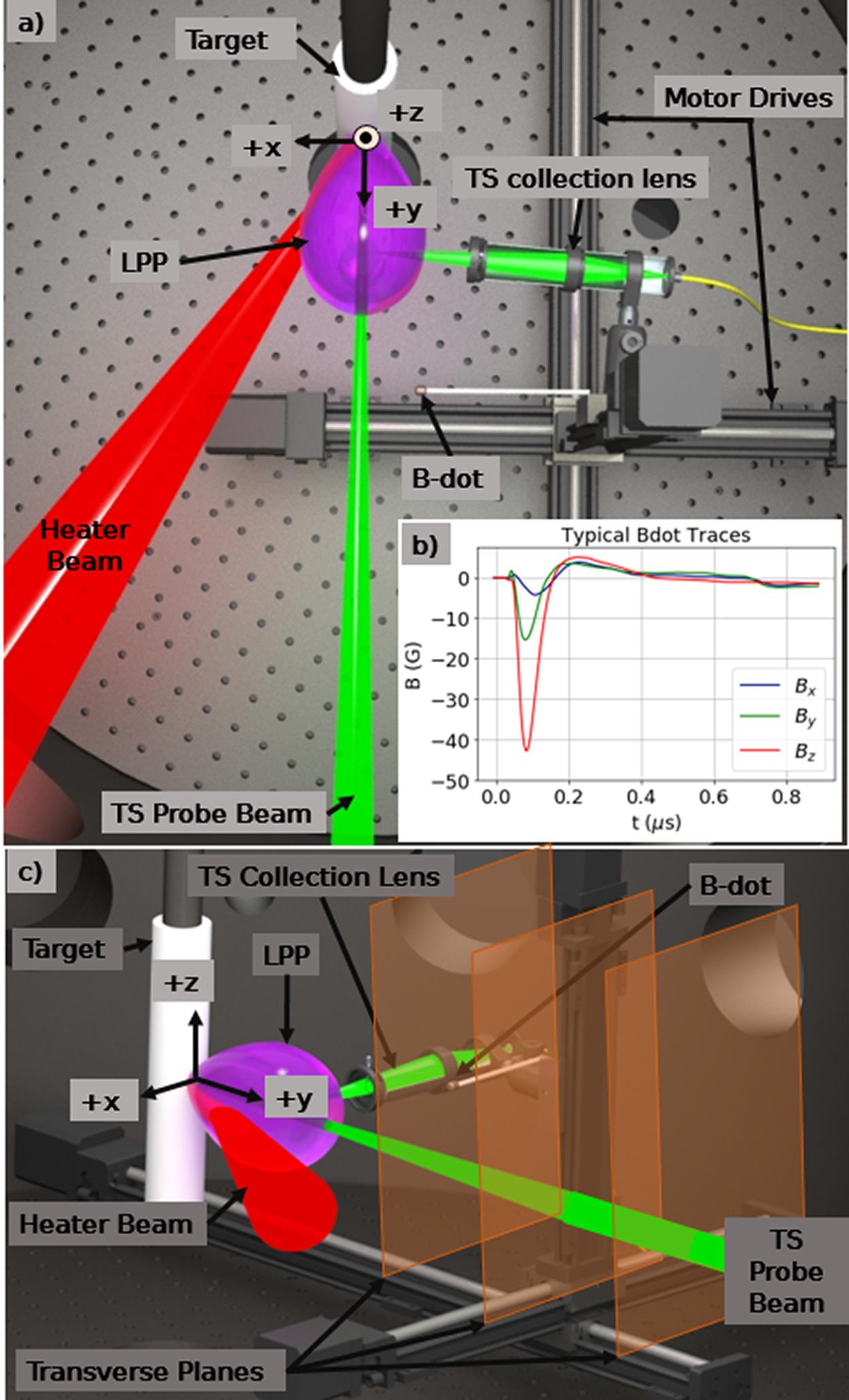
Figure 1.A rendering of the experimental setup. (a) Top view. The origin of the coordinate system is the laser spot on target, with the corresponding axis directions as depicted. (b) Typical B-dot probe traces for all three axes of the probe. (c) Side view. The translucent orange rectangles represent the planes in which magnetic field data were collected.
3 Experimental design
The experimental setup is illustrated in Figure 1. The experiment took place inside a 1 m diameter, stainless steel, cylindrical vacuum chamber. LPPs were created by irradiating a 25 mm diameter cylindrical high-density polyethylene (C2H4) target with a pulsed high-energy heater laser at 34° incidence angle with respect to the target surface normal. The heater laser was a Nd:glass system at 1053 nm wavelength, 15 ns pulse length, with a repetition rate of up to 6 Hz and a maximum output energy of 20 J. The eight-pass amplification scheme involves a phase-conjugation wavefront reversal technique to output a near diffraction-limited spot[31]. In these experiments, the heater laser energy was 10 J and the repetition rate was 1 Hz. The laser was controlled and monitored through a custom-built LabView application that allows automatic synchronization of the laser with the diagnostics and the target motion systems at 1 Hz. The laser was focused down to a 250 μm diameter spot onto the target by an f/25 lens, yielding a nominal intensity of
Measurements of the magnetic field flux were collected using a three-axis magnetic flux (‘B-dot’) probe, the design and construction of which is described in detail elsewhere[32]. The B-dot probe consisted of three sets of thin wire coils wound around three perpendicular axes, each with a diameter of 3 mm. When a magnetic flux passes through the wire coils in the probe, a current is induced. This current is then passed through a differential amplifier and recorded using a digitizer (250 MSamples/s, 125 MHz bandwidth, 12 bit), which recorded for 3.5 μs after the laser shot. The recorded voltage signals are then integrated to yield magnetic field measurements. The integration method used is described in Section 4.
The B-dot probe was mounted on an automated three-axis stepper motor-driven stage inside the chamber. An extensive volumetric scan comprising thousands of shots was created by moving the probe in a pre-defined 3D pattern at a 1 Hz rate with spatial steps of
Due to the direction of the generated fields, we focus on several planes that are perpendicular to the plasma blow-off axis such that we can observe the azimuthal structure of the generated fields. By combining many of these perpendicular planes, we are able to create a 3D picture of the measured Biermann fields. In this experiment, data were collected at the same x and z points in planes at various distances from the target surface along the plasma blow-off axis (y-axis), as illustrated in Figure 1. Each plane was separated from the surrounding planes by a spatial distance of 5 mm.
The plasma temperature and density were measured using optical Thomson scattering[34]. For these measurements, the plasma was probed by a separate 532 nm wavelength probe laser with a 50 mJ output energy and 4 ns pulse width, at a 1 Hz repetition rate. The probe laser enters the chamber along the plasma blow-off axis (
4 Results and analysis
Magnetic flux measurements were taken in multiple planes at varying distances from the target surface. The magnetic flux was calculated from the measured voltage traces using the following integration method, which is described by Everson et al.[32]:
where
![]()
Figure 2.
The position of the B-dot probe was scanned in many transverse planes at distances between 7 and 42 mm from the target surface, each separated by a distance of 5 mm. These planes are pieced together to allow for analysis of the magnetic field structure in three dimensions. A representative portion of the magnetic field data is presented in Figure 2(a). This figure depicts three data planes showing the detected azimuthal magnetic fields,
The magnitude of the largest azimuthal magnetic field detected in each plane decreases with increasing distance from the target (Figure 2(a)). The maximum azimuthal magnetic field values for all planes versus the distance to the plane are shown in Figure 3. A
![]()
Figure 3.Plot of maximum azimuthal magnetic field versus distance from the laser spot. The times at which each point occurs correspond to the times in  curve (red line) agrees well with the data with a value of
  .
.
We calculate the current density
Figure 4 shows a streak plot of the magnetic field at
![]()
Figure 4.A streak plot of the total magnetic field (contour) from a  -lineout at
  mm,
mm,  mm. Linear fits (orange lines) are applied to features of the magnetic field streak plot to determine the speed of different magnetic field features.
![]()
Figure 5.Plot of the maximum of the azimuthal magnetic field observed on the magnetic flux probe (black) at different planes as a function of time. A linear fit (blue line) to the data indicates a speed of 330 km s−1.
Electron temperature and density values were measured using an optical Thomson scattering diagnostic. A single data point at a spatial position of y = 1.5 cm from the heater beam spot along the blow-off axis shows
5 Numerical modeling with FLASH
Ancillary to future measurements that will explore the mechanisms behind the observed return current, and to further interrogate the magnetic field structure in the LPP, we have undertaken a series of simulations using the FLASH code[37]. FLASH is a parallel, multi-physics, adaptive mesh refinement, finite-volume Eulerian hydrodynamics and magnetohydrodynamics (MHD)[38] code, whose high energy density physics capabilities[39] have been validated through benchmarks and code-to-code comparisons[40,41], as well as through direct application to laser-driven laboratory experiments[42–47].
The 2D Cartesian simulation is initialized from a ‘top-down’-perspective of the experimental configuration shown in Figure 1(a). The simulation domain is illustrated in Figure 6(a), modeling the
![]()
Figure 6.(a) Visualization of the 2D simulation domain for the  plane, that is,
  , at
, at  for the laser-facing side of the target. The black semi-circle region denotes the rod that supports the target material (grey). The Peening laser beam enters the simulation domain at a 34° angle from the
  -direction for positive values of
  , reflecting the geometry of the experimental setup provided in
  W at 7.5 ns, which allows 10 J of energy to be deposited to the target over 15 ns as in the experiment.
In our finite-volume, single-fluid Eulerian simulations, the vacuum surrounding the rod must be modeled using a low-density gas. In order to image only the plasma expanding from the target rod, in Figures 7 and 8 we applied two threshold filters to visualize only the LPP properties against a white background. Firstly, we exclude from the visualization cells containing a mass fraction less than 95% of the rod material. Then, we exclude cells whose effective ionization
![]()
Figure 7.Visualization of the FBB 2D FLASH simulation for (a) the electron number density  , (b) the electron temperature
  , (c) the magnitude of the velocity and (d) the magnetic Reynolds number at 150 ns after the laser fires. We describe the threshold applied to these visualizations in the text.
![]()
Figure 8.A visualization of the magnetic field values within the LPP region 150 ns after laser fires. (a) Results from a simulation where the Biermann battery source term was calculated only during the 15 ns duration of the laser (LOBB case) and (b) results where the Biermann battery source term was calculated for the entire simulation duration of 400 ns (FBB case). Provided in (c) are line-outs from (a) LOBB and (b) FBB simulations taken at  cm and
  cm away from the target.
We feature two simulation configurations that aim to determine (1) whether the magnetic fields measured experimentally are consistent with Biermann battery generated magnetic fields, and (2), if so, to quantify the contribution of Biermann battery magnetic field generation in the expanding LPP versus the Biermann battery magnetic fields generated due to the laser–target interaction, which are subsequently advected by the expanding plasma.
In the first simulation, we retain the Biermann battery source term in the induction equation operating throughout the entire simulation duration (i.e., ‘full Biermann battery’ or FBB). In the second simulation, we artificially switch off the Biermann battery source term as soon as the laser pulse ends (i.e., ‘laser-only Biermann battery’ or LOBB). The plasma properties of the ‘realistic’ FBB case are reported in Figure 7, while the resulting magnetic field profiles for both FBB and LOBB simulations are shown in Figure 8. In Figure 7 we report the plasma properties of the LPP predicted by the FLASH FBB simulation. At the region of interest (i.e., the locus of the Thomson scattering measurements), we find electron number densities of the order of
We note the emergence of two plasma lobes near the locus of the laser drive, which are prominently seen in the visualizations of the electron density and temperature (Figures 7(a) and 7(b)). The two lobes surrounding the laser–target spot at the origin and the overall asymmetry of the LPP are caused by the asymmetry of the laser drive via the non-normal incidence angle. One may orient themselves conceptually by considering the bottom most density lobe (
Major points of comparison between Figures 8(a) and 8(b) and the two resulting lineouts, taken at
We speculate that the quantitative discrepancy between the simulation results and the experimental measurements of the electron temperature and velocity can be attributed to the following factors that degrade simulation fidelity: (1) the laser-power temporal profile in the simulation is roughly approximated by a triangular pulse, which alters the deposition rate and the flow dynamics; (2) the FLASH simulations need to be calibrated a posteriori using experimental data to be able to reproduce the laser intensity of the experiment; (3) the spatial resolution of the 2D simulation (
6 Conclusions
We have developed an HRR experimental platform to examine the magnetic fields induced by LPPs over large spatial regions. Data were taken in planes between 0.7 and 4.2 cm from the target surface, revealing azimuthal magnetic fields that reached a peak value of 60 G in the measurement plane closest to the target. The observed fields are azimuthally symmetric, consistent with a simple model of Biermann battery field generation in a cylindrically symmetric LPP. Based on the magnetic Reynolds number,
The current density along the blow-off axis was calculated in each transverse plane via Ampere’s law. The structure of the calculated currents indicates that there is a current loop that forms coincident with the Biermann fields. Further measurements are needed in order to calculate 3D current densities in the system.
Optical Thomson scattering was used to provide measurements of the plasma electron temperature and density at
Future experiments will continue to probe the evolution of the Biermann battery fields over large volumes, allowing us to map 3D regions of spontaneous field generation, as well as regions of advection and diffusion-dominated propagation within the system. Data collection will be expanded to planes further from the target surface and into the gaps between the existing data planes. In addition to increasing the resolution of data collection and expanding the volume over which we probe, we plan to investigate the effects of background gases on spontaneous magnetic field generation.
Further calibration and validation of our FLASH simulations are currently underway. This work will yield improved insights into (1) the coupling of the energy to the target, (2) the magnetic field morphology, (3) the observed potential return current and development of a potential current loop, and (4) set the foundation to study how the plasma properties produced in our experiments affect Biermann battery magnetic field generation. The simulation campaign will also provide a framework for platform design for future experiments.
References
[1] R. M. Kulsrud, E. G. Zweibel. Rep. Progr. Phys., 71, 046901(2008).
[2] R. J. Rand, S. R. Kulkarni. Astrophys. J., 343, 760(1989).
[3] R. Beck. EAS Publ. Ser., 23, 19(2007).
[4] J. L. Han, R. N. Manchester, A. G. Lyne, G. J. Qiao, W. van Straten. Astrophys. J., 642, 868(2006).
[5] E. G. Zweibel, C. Heile. Nature, 385, 131(1997).
[6] C. Heiles. Astrophys. Lett. Commun., 37, 85(1998).
[7] B. A. Remington, R. P. Drake, H. Takabe, D. Arnett. Phys. Plasmas, 7, 1641(2000).
[8] D. D. Ryutov, B. A. Remington, H. F. Robey, R. P. Drake. Phys. Plasmas, 8, 1804(2001).
[9] E. G. Zweibel. Physics, 6, 85(2013).
[10] S. Naoz, R. Narayan. Phys. Rev. Lett., 111, 051303(2013).
[11] G. Gregori, A. Ravasio, C. D. Murphy, K. Schaar, A. Baird, A. R. Bell, A. Benuzzi-Mounaix, R. Bingham, C. Constantin, R. P. Drake, M. Edwards, E. T. Everson, C. D. Gregory, Y. Kuramitsu, W. Lau, J. Mithen, C. Niemann, H.-S. Park, B. A. Remington, B. Reville, A. P. L. Robinson, D. D. Ryutov, Y. Sakawa, S. Yang, N. C. Woolsey, M. Koenig, F. Miniati. Nature, 481, 480(2012).
[12] L. Biermann. Z. Naturforschung, 5, 65(1949).
[13] J. A. Stamper, K. Papadopoulos, R. N. Sudan, S. O. Dean, E. A. McLean, J. A. Dawson. Phys. Rev. Lett., 26, 17(1971).
[14] T. Pisarczyk, S. Y. Gus'kov, R. Dudzak, T. Chodukowski, J. Dostal, N. N. Demchenko, P. Korneev, Z. Kalinowska, M. Kalal, O. Renner, M. Smid, S. Borodziuk, E. Krousky, J. Ullschmied, J. Hrebicek, T. Medrik, J. Golasowski, M. Pfeifer, J. Skala, P. Pisarczyk. Phys. Plasmas, 22, 102706(2015).
[15] A. Gopal, M. Tatarakis, F. N. Beg, E. L. Clark, A. E. Dangor, R. G. Evans, P. A. Norreys, M. S. Wei, M. Zepf, K. Krushelnick. Phys. Plasmas, 15, 122701(2008).
[16] L. L. McKee, R. S. Bird, F. Schwirzke. Phys. Rev. A, 9, 1305(1974).
[17] J. A. Stamper. Laser Particle Beams, 9, 841(1991).
[18] L. Gao, P. M. Nilson, I. V. Igumenshchev, M. G. Haines, D. H. Froula, R. Betti, D. D. Meyerhofer. Phys. Rev. Lett., 114, 215003(2015).
[19] P. M. Nilson, L. Willingale, M. C. Kaluza, C. Kamperidis, S. Minardi, M. S. Wei, P. Fernandes, M. Notley, S. Bandyopadhyay, M. Sherlock, R. J. Kingham, M. Tatarakis, Z. Najmudin, W. Rozmus, R. G. Evans, M. G. Haines, A. E. Dangor, K. Krushelnick. Phys. Rev. Lett., 97, 255001(2006).
[20] G. Gregori, F. Miniati, B. Reville, R. P. Drake. EAS Publ. Series, 58, 23(2012).
[21] C. K. Li, F. H. Séguin, J. R. Rygg, J. A. Frenje, M. Manuel, R. D. Petrasso, R. Betti, J. Delettrez, J. P. Knauer, F. Marshall, D. D. Meyerhofer, D. Shvarts, V. A. Smalyuk, C. Stoeckl, O. L. Landen, R. P. J. Town, C. A. Back, J. D. Kilkenny. Phys. Rev. Lett., 100, 225001(2008).
[22] C. A. Walsh, J. P. Chittenden, K. McGlinchey, N. P. L. Niasse, B. D. Appelbe. Phys. Rev. Lett., 118, 155001(2017).
[23] P. T. Campbell, C. A. Walsh, B. K. Russell, J. P. Chittenden, A. Crilly, G. Fiksel, P. M. Nilson, A. G. R. Thomas, K. Krushelnick, L. Willingale. Phys. Rev. Lett., 125, 145001(2020).
[24] S. I. Braginskii. Rev. Plasma Phys., 1, 205(1965).
[25] R. S. Craxton, M. G. Haines. Phys. Rev. Lett., 35, 20(1975).
[26] R. S. Craxton, M. G. Haines. Plasma Phys., 20, 487(1978).
[27] A. Raven, O. Willi, P. T. Rumsby. Phys. Rev. Lett., 41, 554(1978).
[28] M. G. Haines. Canad. J. Phys., 64, 912(1986).
[29] E. A. McLean, J. A. Stamper, C. K. Manka, H. R. Griem, D. W. Droemer, B. H. Ripin. Phys. Fluids, 27, 1327(1984).
[30] R. S. Bird, L. L. McKee, F. Schwirzke, A. W. Cooper. Phys. Rev. A, 7, 1328(1973).
[31] C. B. Dane, L. E. Zapata, W. A. Neuman, M. A. Norton, L. A. Hackel. IEEE J. Quantum Electron., 31, 148(1995).
[32] E. T. Everson, P. Pribyl, C. G. Constantin, A. Zylstra, D. B. Schaeffer, N. L. Kugland, C. Niemann. Rev. Sci. Instrum., 80, 113505(2009).
[33] D. B. Schaeffer, L. R. Hofer, E. N. Knall, P. V. Heuer, C. G. Constantin, C. Niemann. High Power Laser Sci. Eng., 6, e17(2018).
[34] D. H. Froula, S. H. Glenzer, N. C. Luhmann, J. Sheffield, T. J. H. Donné. Fusion Sci. Technol., 61, 104(2012).
[35] M. Kaloyan, S. Ghazaryan, C. G. Constantin, R. S. Dorst, P. V. Heuer, J. J. Pilgram, D. B. Schaeffer, C. Niemann. Rev. Sci. Instrum., 92, 093102(2021).
[36] D. B. Schaeffer, A. S. Bondarenko, E. T. Everson, S. E. Clark, C. G. Constantin, C. Niemann. J. Appl. Phys., 120, 043301(2016).
[37] B. Fryxell, K. Olson, P. Ricker, F. X. Timmes, M. Zingale, D. Q. Lamb, P. MacNeice, R. Rosner, J. W. Truran, H. Tufo. Astrophys. J. Suppl. Ser., 131, 273(2000).
[38] D. Lee. J. Comput. Phys., 243, 269(2013).
[39] P. Tzeferacos, M. Fatenejad, N. Flocke, C. Graziani, G. Gregori, D. Q. Lamb, D. Lee, J. Meinecke, A. M. Scopatz, K. Weide. High Energy Density Phys., 17, 24(2015).
[40] M. Fatenejad, B. Fryxell, J. Wohlbier, E. Myra, D. Lamb, C. Fryer, C. Graziani. High Energy Density Phys., 9, 63(2013).
[41] C. Orban, M. Fatenejad, S. Chawla, S. C. Wilks, D. Q. Lamb. , , , , and , arXiv:1306.1584 ().(2013).
[42] J. Meinecke, H. W. Doyle, F. Miniati, A. R. Bell, R. Bingham, R. Crowston, R. P. Drake, M. Fatenejad, M. Koenig, Y. Kuramitsu, C. C. Kuranz, D. Q. Lamb, D. Lee, M. J. MacDonald, C. D. Murphy, H.-S. Park, A. Pelka, A. Ravasio, Y. Sakawa, A. A. Schekochihin, A. Scopatz, P. Tzeferacos, W. C. Wan, N. C. Woolsey, R. Yurchak, B. Reville, G. Gregori. Nat. Phys., 10, 520(2014).
[43] J. Meinecke, P. Tzeferacos, A. Bell, R. Bingham, R. Clarke, E. Churazov, R. Crowston, H. Doyle, R. P. Drake, R. Heathcote, M. Koenig, Y. Kuramitsu, C. Kuranz, D. Lee, M. MacDonald, C. Murphy, M. Notley, H.-S. Park, A. Pelka, A. Ravasio, B. Reville, Y. Sakawa, W. Wan, N. Woolsey, R. Yurchak, F. Miniati, A. Schekochihin, D. Lamb, G. Gregori. Proc. Natl. Acad. Sci. USA, 112, 8211(2015).
[44] C. K. Li, P. Tzeferacos, D. Lamb, G. Gregori, P. A. Norreys, M. J. Rosenberg, R. K. Follett, D. H. Froula, M. Koenig, F. H. Seguin, J. A. Frenje, H. G. Rinderknecht, H. Sio, A. B. Zylstra, R. D. Petrasso, P. A. Amendt, H. S. Park, B. A. Remington, D. D. Ryutov, S. C. Wilks, R. Betti, A. Frank, S. X. Hu, T. C. Sangster, P. Hartigan, R. P. Drake, C. C. Kuranz, S. V. Lebedev, N. C. Woolsey. Nat. Commun., 7, 13081(2016).
[45] P. Tzeferacos, A. Rigby, A. F. A. Bott, A. R. Bell, R. Bingham, A. Casner, F. Cattaneo, E. M. Churazov, J. Emig, F. Fiuza, C. B. Forest, J. Foster, C. Graziani, J. Katz, M. Koenig, C.-K. Li, J. Meinecke, R. Petrasso, H.-S. Park, B. A. Remington, J. S. Ross, D. Ryu, D. Ryutov, T. G. White, B. Reville, F. Miniati, A. A. Schekochihin, D. Q. Lamb, D. H. Froula, G. Gregori. Nat. Commun., 9, 591(2018).
[46] L. E. Chen, A. F. A. Bott, P. Tzeferacos, A. Rigby, A. Bell, R. Bingham, C. Graziani, J. Katz, M. Koenig, C. K. Li. Astrophys. J., 892, 114(2020).
[47] A. F. A. Bott, P. Tzeferacos, L. Chen, C. A. J. Palmer, A. Rigby, A. R. Bell, R. Bingham, A. Birkel, C. Graziani, D. H. Froula, J. Katz, M. Koenig, M. W. Kunz, C. Li, J. Meinecke, F. Miniati, R. Petrasso, H.-S. Park, B. A. Remington, B. Reville, J. S. Ross, D. Ryu, D. Ryu, F. H. Séguin, T. G. White, A. A. Schekochihin, D. Q. Lamb, G. Gregori. Proc. Natl. Acad. Sci. USA, 118, e2015729118(2021).
[48] M. Fatenejad, A. R. Bell, A. Benuzzi-Mounaix, R. Crowston, R. P. Drake, N. Flocke, G. Gregori, M. Koenig, C. Krauland, D. Lamb, D. Lee, J. R. Marques, J. Meinecke, F. Miniati, C. D. Murphy, H.-S. Park, A. Pelka, A. Ravasio, B. Remington, B. Reville, A. Scopatz, P. Tzeferacos, K. Weide, N. Woolsey, R. Young, R. Yurchak. High Energy Density Phys., 9, 172(2013).


Set citation alerts for the article
Please enter your email address

© Copyright 2018-2021 | Chinese Laser Press. All Rights Reserved 沪ICP备15018463号-20