Two-photon absorption (TPA)^[1–5] is a kind of photonic approach, as a quadratic response to the incident optical intensity. Recently, TPA in semiconductors is employed to measure optical autocorrelation due to similar sensitivity and potential low-cost compared to a second-harmonic generation (SHG) crystal^[6] autocorrelator. In the previous work^[7], it is expounded that Si and GaAs photodiodes can be used as TPA devices for autocorrelation measurement of laser pulses at 1550 nm. The difference between Si and GaAs is mainly compared for dispersive pulses measurement. Compared with Si, GaAs is a direct gap semiconductor material whose electronic energy level transition does not involve the simultaneous emission or absorption of a phonon, and TPA has been observed experimentally to be stronger in GaAs presently^[8,9]. Therefore, GaAs can be preferred in autocorrelation measurements in order to avoid the influence of the environment.

Both the intensity and interferometric autocorrelation cannot retrieve the pulse information (intensity and phase) completely. They are not sufficient to determine the temporal profile of the pulse, but we can curve-fit the autocorrelation signal to measure the pulse duration. For traditional fitting methods such as the Levenberg–Marquardt (L-M) method, we need to preset the pulse function in advance. A measured autocorrelation signal cannot be the perfect Gauss or sech² shape due to the influence of the electronic noise, which could result in bad fitting. In recent years, with the development of deep learning, neural networks (NNs) have shined in public security, national defense, and industry. The universal approximation theorem^[10,11] shows that any function can be theoretically approximated by NNs with at least one hidden layer. It shows its unique advantages in curve-fitting.

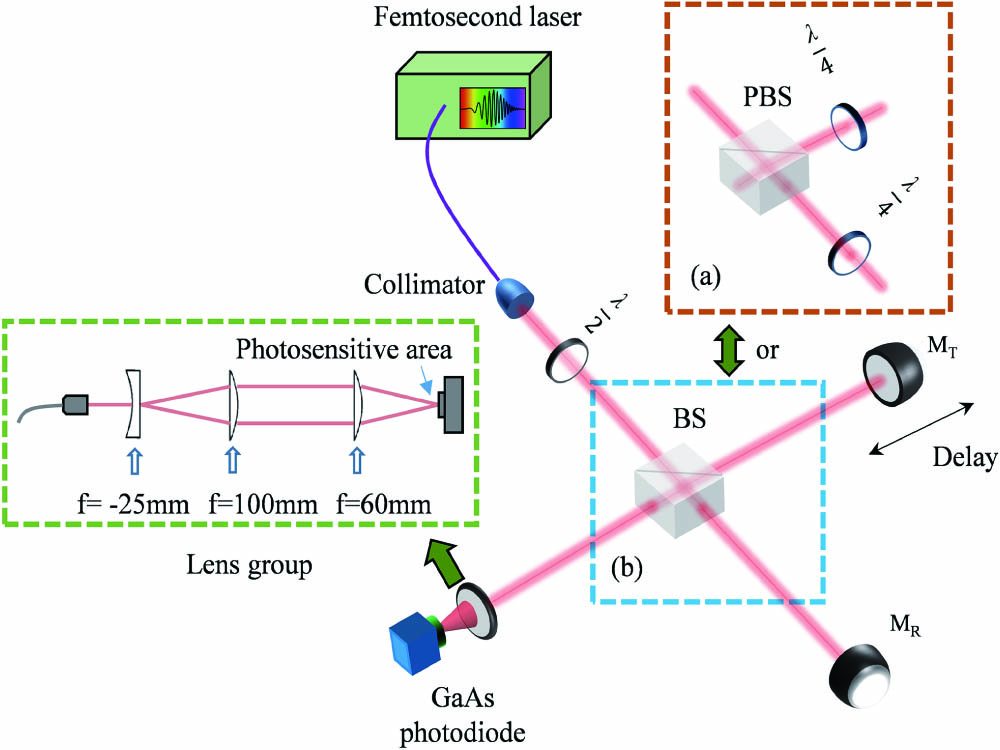
In this work, we focus on measuring the temporal profile of pulses at 1550 nm from an erbium-doped fiber laser using an NN method. A photodiode-based autocorrelation measurement experiment system using a Michelson interferometer configuration is shown in Fig. 1. For the intensity autocorrelation measurement [Fig. 1(a)], a single sequence of pulses is split into two orthogonally polarized parts (O part and E part) with the same intensity by the half-wave plate and polarizing beam splitter (PBS). The light of the O part propagates into the reference arm and is reflected by the reference corner cube MR, while the light of the E part is transmitted into the scanning arm and reflected by the other corner cube MT mounted on a movable stage. Quarter-wave plates between the PBS and cubes can tune the polarization of the beams, avoiding the interference. For Fig. 1(b), the PBS is replaced by a beam splitter (BS), and all of the plates are removed. Without the control of the polarization, interferometric autocorrelation will occur in this configuration. For a strong TPA effect, we place an objective lens group between the PBS (or BS) and the photodiode to focus laser pulses onto the photosensitive area of the photodiode.

In the interferometric autocorrelation optical configuration, the optical intensity of the recombined pulses can be expressed as where E(t) and E(t−τ) denote the optical fields of the reference and scanning laser pulses, respectively. τ represents the time delay between two sequences of pulses.

When two sequences of pulses from the same laser recombine at the photosensitive area of the photodiode, twice the photon energy exceeds the semiconductor energy gap, and a strong TPA can be excited. Hence, the voltage signal induced by TPA is associated with the square of the incident light intensity as where m is an intensity coefficient related to the photosensitive area of the photodiode, the equivalent capacitance of the photodiode with bias voltage, and the TPA coefficient. Thus, the measured interferometric autocorrelation trace can be obtained as a function of the delay,

The first term is a constant that is uninteresting for us. The second term represents the intensity autocorrelation, which can be extracted by a fitting method. The third term considers the oscillations at ω in delay, which is the sum-of-intensities-weighted interferogram of E(t). The fourth term is the interferogram of the second harmonic, equivalent to the spectrum of the second harmonic (oscillations at 2ω in delay).

For pulse width inferring, we can import the intensity autocorrelation part of Eq. (3) into an NN for the curve-fitting. Figure 2 shows the basic process of machine learning and an example of a simple typical NN. A typical machine learning process includes target determination (determine the model prediction target), data cleaning (handle invalid and missing values), model building (choose the right machine learning model), model training (update model parameters continuously by using the data), and model application (achieve goal prediction by using the model). To build an NN model, as shown in Fig. 2(b), we should set up the input layer, hidden layer, and output layer, and the number of neurons and activation function of each layer should be determined appropriately. The input data (x0,…,xi,…,xn) feed forward to produce the output data, and the output error is in back propagation with the target data y to modify the parameters of the model.

If we define τ as the network input, which is the time delay series of the detected autocorrelation signal, the network output can be simplified to where w1i and wiY are the weights of the network, and gi is the Sigmod function for hidden neurons. Here, we define N as epochs of the NN. Mathematically gi can be described by the equation

The network is then trained using a set of two-dimensional arrays containing input–output pairs (xi,yi) with xi and yi representing the time data and corresponding value data of the desired autocorrelation function. Often it is convenient to use the least square method when evaluating the quality of the network, that is,

Finally, the weight and bias are automatically updated in the network through back propagation and gradient descent. When the threshold condition (performance or epochs) is reached, a model suitable for signal-fitting is formed.

Experimental observations of the interferometric autocorrelation are performed to test the TPA-based autocorrelator. A nonlinear polarization rotation (NPR) mode-locked erbium-doped fiber laser (C-fiber 1550, Menlo System) is used to generate pulses in the experiment. It produces about 30 mW, 88 fs pulses. A GaAs photodiode is used to generate TPA, and its photosensitive area is about 500 μm. A linear stage (M-521.DD, Physik Instrument Co., Germany) with a 200 mm movement range and 0.1 μm resolution is used to generate the delay in the experimental system.

Here, we use the configuration in Fig. 1(b). A measured GaAs-based interferometric autocorrelation trace is plotted in Fig. 3(a). To calibrate the pulse duration, femtosecond laser pulses are coupled into a commercial autocorrelator based on the conventional SHG crystal [pulseCheck universal serial bus (USB), Angewandte Physik & Elektronik GmbH]. The interferometric autocorrelation curve is obtained by pulseCheck USB as shown in Fig. 3(b) for comparison. For the interferometric autocorrelation measurement, the TPA effect in the GaAs photodiode is in excellent agreement with the traditional SHG.

To further retrieve the pulse width information, the TPA-based autocorrelation function of the laser pulse is measured by an NN method with the intensity autocorrelation experimental configuration. Here, we build an NN with two hidden layers. The PyTorch kit in Python is used to generate the NN, and the number of neurons in each hidden layer is set to 10. The performance parameter refers to the maximum value of the mean square error (MSE). If the current MSE is less than the set value, the training is stopped. This indicator can be set with the trainParam.goal parameter. When the performance is set, the corresponding parameters gradient, momentum constant (μ), and validation checks are generated. The gradient parameter represents the current gradient value in the gradient descent method. If the current gradient value reaches the set value, the training is stopped. μ also stands for momentum parameter, which is included in the weight update expression to avoid the problem of local minimum. Sometimes the network may get stuck to the local minimum and the convergence does not occur. The range of μ is between 0 and 1. The validation checks parameter is a generalization ability check. If the training error does not decrease but rises for six consecutive times, the training is forcibly ended.

For the curve-fitting, we just set the number of neurons in the input and output layer to one. Respectively, we select the transfer function of the hidden layer as tansig, the transfer function of the output layer as purelin, and the learning algorithm as trainlm. The size of the input and label data is a 1×10,000array, corresponding to the sampling number of the autocorrelation signal. The epochs are set as 10,000, and we train the model at four performance values of 10−5, 10−6, 10−7, and 10−8. The curve-fitted autocorrelation traces are depicted in Fig. 4. That is to say, when the performance is improved to about 10−7, we can get a nice curve-fitting. The FWHM of the fitted autocorrelation function is calculated as about 124.18 fs with the performance of 10−7.

The training process is represented in Fig. 5. Overall, the entire training process did not fall into the local optimum. The training ends at epoch 547, while the performance reaches 10−7. Figure 5(a) shows the training state, including the update process of the parameter gradient, μ, and validation checks. The gradient generally updates with a downward trend. The μ parameter floats in the normal range. During the training process, the validation check has been kept at a value of zero, indicating that the model training is very successful. The best training performance is 1.3096×10−7 at epoch 547, as shown in Fig. 5(b). At last, to show the performance of the fitting, in Fig. 5(c), the target and output of the model are compared using the regression analysis. The structure of the NN for this measurement system is shown in Fig. 5(d). The relationship between the target and output can be linear-fitted by where Target and Output represent the real and predicted signal. R of the regression is calculated as about 0.91642.

The resolution in the pulse duration measurement mainly depends on the translation step size of the stage used to generate the variable delay. The uncertainty can be deduced by 2δs=c·δτ, where δs is the positioning accuracy. The movement resolution is 0.1 μm here corresponding to a delay resolution of about 0.7 fs. The average error of the measured FWHM of the fitted autocorrelation function is recorded as 0.9 fs with the performance of 10−8, and 1.1 fs with the performance of 10−7. Experimental results coincide with the theoretical analysis. Furthermore, setting a better performance can achieve a better fitting, but it will cost more model training time. So, we should choose the right performance, considering not only a higher performance for NN.

To further compare the performance of L-M and NN, the autocorrelation trace was Gaussian-fitted using the normal L-M fitting method. Due to the effect of the noise, bad fitting occurs, as shown in Fig. 6(a). Here, a set of test pulses is selected, and two out of every 10 signals have bad fitting on average. Similarly, a normal L-M fitting is compared in Fig. 6(b). It is easily seen that the bad fitting may occur with the L-M method, when the autocorrelation signal contains some slight noise. Obviously, NN can restore the intensity autocorrelation trace well, regardless of the noise. However, the normal L-M fitting performs worse for the signal with the noise. Thus, for pulse width inferring, NN is a better choice.

It is clear that both L-M and NN can curve-fit autocorrelation traces in pulse duration measurements. However, L-M needs to preset the type of fitting functions, so it is too sensitive to the shape matching of the actual signal, which reduces the success rate of the fitting substantially. Furthermore, L-M gets a weak ability to fit the signal with the noise, and it can be easily misguided by the noise. NN can solve these problems very well. With appropriate neurons and layers, NNs can generate arbitrary functions. In this way, there is no need to preset the fitting function, and it can still fit the autocorrelation trace well in the presence of noise. Therefore, NN is preferable for the laser pulse duration measurement to improve the robustness of the autocorrelator.

In summary, we develop a TPA-based temporal profile inferring method of the erbium-doped fiber laser pulses at 1550 nm using an NN method. NN can retrieve the intensity autocorrelation function extremely accurately and has a certain noise reduction ability, simplifying the signal processing process for a TPA photodiode-based autocorrelator.

References

[1] J. Ma, J. Chiles, Y. D. Sharma, S. Krishna, S. Fathpour. Opt. Lett., 39, 5297(2014).
[2] S. Fathpour, K. Tsia, B. Jalali. Appl. Phys. Lett., 89, 061109(2006).
[3] Y. Xie, S. Zhang, X. Zhang, N. Dong, I. M. Kislyakov, S. Luo, Z. Chen, J. Nunzi, L. Zhang, J. Wang. Chin. Opt. Lett., 17, 081901(2019).
[4] M. K. Lee, C. H. Chu, Y. H. Wang, S. M. Sze. Opt. Lett., 26, 160(2001).
[5] S. I. Shin, Y. S. Lim. J. Opt. Soc. Korea., 20, 435(2016).
[6] X. Wang, H. Ren, G. Wang, J. He. Chin. Opt. Lett., 17, 081902(2019).
[7] J. Chen, W. Xia, M. Wang. J. Appl. Phys., 121, 223103(2017).
[8] A. Villeneuve, C. C. Yang, G. I. Stegeman, C. N. Ironside, G. Scelsi, R. M. Osgood. IEEE J. Quantum Electron., 30, 1172(1994).
[9] S. Krishnamurthy, Z. G. Yu, L. P. Gonzalez, S. Guha. J. Appl. Phys., 109, 033102(2011).
[10] G. Cybenko. Math. Control Signals Syst., 2, 303(1989).
[11] K. Hornik. Neural Networks, 4, 251(1991).