Optomagnonic frequency combs

Zeng-Xing Liu; Yong-Qing Li

doi:10.1364/PRJ.467595

Abstract

Optical frequency combs are fundamentally important in precision measurement physics, bringing unprecedented capabilities of measurements for time keeping, metrology, and spectroscopy. In this work, we investigate theoretically the formation of a form of frequency combs in cavity optomagnonics, in which a ferrimagnetic insulator sphere supports optical whispering gallery modes for both light photons and magnons. Numerical simulations of the optomagnonic dynamics show that a robust frequency comb can be obtained at low power under the bichromatic pumping drive, and the comb spacing is adjustable. Furthermore, the optomagnonic frequency comb structure has abundant non-perturbative features, suggesting that the magnon-induced Brillouin light scattering process in cavity optomagnonics may also exhibit phenomena similar to those in atomic–molecular systems. In addition to providing insight into optomagnonic nonlinearity, optomagnonic frequency combs may also provide the feasibility of implementing frequency combs based on spintronic platforms and may find applications for precision metrology based on magnonic devices.

1. INTRODUCTION

A frequency comb is a spectrum composed of a series of evenly spaced and discrete frequency components with coherent and stable phase relationships [1 –9]. It has been extensively studied and has had a broad impact on fundamental science and advanced technology, such as optical metrology [2], precision spectroscopy [3], optical atomic clocks [4], molecular fingerprinting [5], and astrophysical spectrometers calibration [6]. With the development of research, many methods to generate frequency combs have been proposed. For example, the conventional optical frequency combs are implemented in optical systems based on mode-locked lasers [1] and later realized in chip-scale microresonators mediated via the Kerr nonlinearity [7,8], which has the potential to make frequency metrology and spectroscopy widely applicative. In addition, a direct analog of frequency combs in the phononic domain has been reported in a microscopic extensional mode resonator via three-mixing process [10,11]. More recently, frequency combs have also been theoretically predicted and experimentally proved in the area of spin waves [12 –14].

Magnons, the quasiparticle of spin-wave excitations in ordered magnets, have become a widely applicative research topic in the field of condensed matter physics and quantum optics [15 –35]. As a fundamentally different type of light–matter interaction, cavity optomagnonics has attracted much attention, and is the study of the cavity-enhanced interaction between optical photons and magnons via spin–orbit coupling [29 –35]. Cavity optomagnonics provides a powerful methodology for the coherent control of spin waves using light, which emerges as a promising candidate for efficient microwave-to-optics transduction [36,37]. Moreover, many photonic phenomena, such as optical cooling of magnons [38], magnon heralding [39], and magnon lasers [40 –42], have been reported in cavity optomagnonics. Despite the similarities between magnons and photons in many aspects, a direct analog for optical frequency combs in cavity optomagnonics has not yet been well studied.

The purpose of the present work is to investigate a novel frequency comb in the optomagnonics domain, in which the magnon-mediated Brillouin scattering between optical photons and magnons induces the generation of optomagnonic frequency combs. The frequency $ω$ of the $n$ th comb tooth can be written as a simple function of two frequencies: pumping frequency $ω_{l}$ and repetition frequency $ω_{r}$ , such that $ω = ω_{l} \pm n ω_{r}$ . Our theory shows that using bichromatic pumping to generate frequency combs has its inherent advantages, such as low power, robust frequency comb teeth, and adjustable comb spacing. Also, the non-perturbative features of optomagnonic frequency combs are discussed in detail, suggesting that the magnon mode may also exhibit phenomena that are similar to those in atomic–molecular systems [43 –45], including non-perturbative effects. In addition, the feasibility of experimental observation of optomagnonic frequency combs under current experimental conditions has been evaluated [30 –32,36,46]. Beyond their fundamental scientific significance, our results provide a new idea for exploring novel types of frequency combs in the optomagnonics domain and may find potential applications in precision metrology based on magnonic devices [47 –49].

Sign up for Photonics Research TOC. Get the latest issue of Photonics Research delivered right to you！Sign up now

2. MODEL AND THEORY

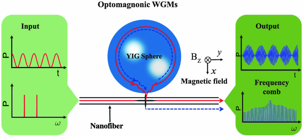
The physical model we consider is a cavity optomagnonics system, as shown in Fig. 1, in which a ferromagnetic insulator yttrium iron garnet (YIG) sphere supports whispering gallery modes (WGMs) for light photons, as well as the magnetostatic mode for magnons with a frequency $ω_{m}$ . To saturate the magnetization, an external magnetic field $B_{z}$ perpendicular to the WGM orbital plane ( $x - y$ plane) is introduced. The frequency of the magnon mode in the YIG sphere can be tuned by adjusting the external magnetic field, i.e., $ω_{m} = ϱ B_{m}$ , where $ϱ / 2 π = 28 GHz / T$ is the gyromagnetic ratio, and $B_{m}$ is the magnetic field strength [50]. The input laser is introduced through a polarization controller and then evanescently coupled to the YIG sphere via a tapered optical nanofiber, and light is confined within the symmetrical sphere due to the complete internal reflection, forming a WGM resonator [30 –32]. Of particular note is that the waveguide is assumed to be a single-mode fiber that supports only one transverse optical mode with two polarization components, $E ∥ z$ or $E ∥ x$ , marked as transverse-electric (TM) mode and transverse-magnetic (TE) mode, respectively. Furthermore, assuming that the direction of light propagation ( $x - y$ plane) is perpendicular to the mean magnetization in ferromagnets ( $z$ direction), the well-known magnon-induced Brillouin scattering will occur [51]. Brillouin scattering is essentially the inelastic scattering of light excited by various quasiparticles, such as polarons, phonons, or magnons [52]. For the cavity optomagnonic system, the photons in the WGM resonator and the magnons in the YIG sphere undergo Brillouin scattering to produce Stokes photons or anti-Stokes photons. Under weak excitation, the Hamiltonian of the cavity optomagnonic system, including the optical part, the magnetic subsystem, and the optomagnonic interaction, can be described as [29] $H_{COM} = H_{opt} + H_{mag} + H_{int},$ (1)where $H_{opt} = \int [\sum_{ı j} \frac{ϵ_{ı j} (M_{s})}{2} E_{ı} E_{j}^{*} + \frac{| B_{L} |^{2}}{2 μ_{0}}] d r, H_{mag} = \int [- ϱ M \cdot (B_{0} e_{z} + B_{d}) + \frac{{| B_{d} |}^{2}}{2 μ_{0}}] d r, H_{int} = \sum_{ı j} \int \frac{ϵ_{ı j} (M)}{2} E_{ı} E_{j}^{*} d r .$ (2) $ϵ_{ı j} (M_{s})$ and $ϵ_{ı j} (M)$ are, respectively, the elastic and inelastic terms of the dielectric permittivity tensor, where $ı, j \in {x, y, z}$ . $E_{ı (j)}$ denotes the component of the electric field, and $μ_{0}$ is the vacuum magnetic permeability. $B = B_{0} e_{z} + B_{L} + B_{d}$ is the total magnetic field with $B_{0}$ the dc applied static magnetic field in the $z$ direction that saturates the magnetization, $B_{L}$ the ac contribution due to light at optical frequencies, and $B_{d}$ the demagnetizing field induced by the static magnetic field [33]. $M = (M_{x}, M_{y}, M_{z})$ represents the magnetization of the YIG sphere, with the macrospin operator introduced, i.e., the relation $S = M V_{m} / ϱ \equiv (S_{x}, S_{y}, S_{z})$ , where $V_{m}$ is the volume of the YIG sphere. Hence, the Hamiltonian in Eq. (1), in quantum mechanical language, can be quantized as $H_{COM} = ℏ ω_{a} a^{†} a + ℏ ω_{b} b^{†} b - γ B_{0} S_{z} + ℏ g (S_{+} a b^{†} + S_{-} a^{†} b) + h.c.,$ (3)where $a$ ( $a^{†}$ ) and $b$ ( $b^{†}$ ) are the annihilation (creation) operators of the optical TM and TE modes with frequencies $ω_{a}$ and $ω_{b}$ , respectively. $g = \frac{1}{N_{spin}} \frac{c}{n_{r}} V$ is the optomagnonic coupling coefficient with $N_{spin}$ the number of spins in the YIG sphere, $V$ the Verdet constant, $n_{r}$ the refractive index, and $c$ the vacuum speed of light [31]. Assume that the direction of the dc magnetic field is in the $z$ direction; thereby, the raising and lowering operators of the macrospin $S_{\pm} \equiv S_{x} \pm i S_{y}$ can be introduced via the Holstein–Primakoff transformations [53] $S_{+} = (\sqrt{2 S - m^{†} m}) m, S_{-} = m^{†} (\sqrt{2 S - m^{†} m}), S_{z} = S - m^{†} m,$ (4)where $S$ is the total spin number of the macrospin operator, and $m$ $(m^{†})$ is the annihilation (creation) operator of the magnon mode. For low-lying excitations, i.e., the generated magnon number is much smaller than the total spin number $⟨ m^{†} m ⟩ / 2 S ≪ 1$ , the macrospin operators can be approximated by $S_{+} \approx \sqrt{2 S} m$ and $S_{-} \approx m^{†} \sqrt{2 S}$ . The Hamiltonian in Eq. (3), therefore, can be obtained as $H_{COM} = ℏ ω_{a} a^{†} a + ℏ ω_{b} b^{†} b + ℏ ω_{m} m^{†} m + ℏ g (a b^{†} m + a^{†} b m^{†}),$ (5)where $g = \sqrt{2 S} g = V \frac{c}{n_{r}} \sqrt{\frac{2}{n_{spin} V_{m}}}$ is the effective optomagnonic coupling strength with $n_{spin}$ the spin density. For a YIG sphere with a diameter of 200 μm, the effective optomagnonic coupling strength is theoretically evaluated to be $g_{0} = 2 π \times 39.2 Hz$ [54].

Figure 1.Schematic illustration of the optomagnonic WGMs, in which the YIG sphere supports WGMs for photons and the magnetostatic mode for magnons. A magnetic field $B_{z}$ perpendicular to the plane of the WGM is applied to saturate the magnetization. A bichromatic input laser light (temporal and spectral in the rotating frame) evanescently couples to the optical WGMs via a nanofiber, and the output field supports the generation of optomagnonic frequency combs.

Suppose that the input laser, including a driving field and a probe field with powers $P_{l}$ and $P_{p}$ and frequencies $ω_{l}$ and $ω_{p}$ , is adjusted to couple to the TM mode. Furthermore, a hypothesis that Brillouin scattering occurs only between TM and TE modes with the same WGM index is also taken into account [29]. Simultaneously, the YIG sphere is pumped by a microwave incident field with pump power $P_{m}$ and frequency $ω_{m w}$ . Thus, the total time-dependent Hamiltonian can be written as $H_{tot} = ℏ ω_{a} a^{†} a + ℏ ω_{b} b^{†} b + ℏ ω_{m} m^{†} m + ℏ g (a b^{†} m + a^{†} b m^{†}) + ℏ ϵ_{l} (a e^{i ω_{l} t} + a^{†} e^{- i ω_{l} t}) + ℏ ϵ_{p} (a e^{i ω_{p} t} + a^{†} e^{- i ω_{p} t}) + ℏ ϵ_{m} (m e^{i ω_{mw} t} + m^{†} e^{- i ω_{mw} t}),$ (6)where $ϵ_{l (p) (m)} = \sqrt{2 κ_{a (m)} P_{l (p) (m w)} / ℏ ω_{l (p) (m w)}}$ is the Rabi frequency denoting the coupling strength between the optical (microwave) driving field and TM optical (magnon) mode. $κ_{a}$ and $κ_{m}$ are the decay rates of the TM optical mode and magnon mode, respectively. To make the driving terms time independent, a doubly rotating frame for the optical and microwave driving frequencies is adopted. Namely, applying the unitary transformation $U (t) = \exp [- i ω_{l} a^{†} a t - i ω_{m w} m^{†} m t - i (ω_{l} + ω_{m w}) b^{†} b t]$ , the Hamiltonian in Eq. (6) can be written in the form $H_{tot} = U (t) H U^{†} (t) - i ℏ U (t) \frac{\partial U^{†} (t)}{\partial t} = ℏ Δ_{a} a^{†} a + ℏ Δ_{b} b^{†} b + ℏ Δ_{m} m^{†} m + ℏ g (a b^{†} m + a^{†} b m^{†}) + ℏ ϵ_{l} (a + a^{†}) + ℏ ϵ_{p} (a e^{i Δ_{p} t} + a^{†} e^{- i Δ_{p} t}) + ℏ ϵ_{m} (m + m^{†}),$ (7)where $Δ_{a} = ω_{a} - ω_{l}$ and $Δ_{b} = ω_{b} - ω_{l} - ω_{m w}$ are the detunings between the optical driving frequency and the TM and TE optical modes, respectively. In addition, $Δ_{m} = ω_{m} - ω_{m w}$ is the detuning from the microwave pumping field and the magnon mode, and $Δ_{p} = ω_{p} - ω_{l}$ is the beat frequency between the optical driving field and the probe field. It should be noted that the optomagnonic interaction, similar to the optomechanical interaction [55], is inherently nonlinear, which becomes clear after taking the following transformation: $H_{Kerr} = U^{†} H_{COM} U = ℏ ω_{a} a^{†} a + ℏ ω_{b} b^{†} b + ℏ ω_{m} m^{†} m + ℏ \frac{g^{2}}{ω_{m}} a^{†} b a b^{†}$ , where the unitary $U = \exp [(m^{†} - m) (g / ω_{m}) a^{†} b]$ . Obviously, it can be seen that the mutual effects between the optical and magnon modes can be seen as cross-Kerr-like nonlinear interaction.

According to the Heisenberg–Langevin approach, the dynamic behavior of the cavity optomagnonic system can be described by the following nonlinear equations: $□ \cdot Φ = M Φ - i μ + ϱ,$ (8)where $□ \cdot Φ = \frac{d}{d t} {(a, b, m)}^{T}$ , $Φ = {(a, b, m)}^{T}$ , $μ = {(ε_{l} + ϵ_{p} e^{- i Δ_{p} t},0, ε_{m})}^{T}$ , and $M = (\begin{matrix} - (i Δ_{a} + κ_{a}) & - i g m^{†} & 0 \\ 0 & - (i Δ_{b} + κ_{b}) & - i g a \\ 0 & - i g a^{†} & - (i Δ_{m} + κ_{m}) \end{matrix}),$ where $κ_{b}$ is the damping rate of the TE optical mode, and for simplicity, we assume that TM and TE optical modes have identical damping rates $κ_{a} = κ_{b}$ . $ϱ = (\sqrt{2 κ_{a}} a_{i n} (t), \sqrt{2 κ_{b}} b_{i n} (t), \sqrt{2 κ_{m}} m_{i n} (t {))}^{T}$ represent the noise terms of the optical and magnon modes, characterized by the temperature-dependent correlation functions [56] $⟨ a_{in} (t) a_{in}^{†} (t^{'}) ⟩ = [n_{th} (ω_{a}) + 1] δ (t - t^{'})$ , $⟨ a_{in}^{†} (t) a_{in} (t^{'}) ⟩ = [n_{th} (ω_{a})] δ (t - t^{'})$ , and $⟨ m_{in} (t) m_{in}^{†} (t^{'}) ⟩ = [m_{th} (ω_{m}) + 1] δ (t - t^{'})$ , $⟨ m_{in}^{†} (t) m_{in} (t^{'}) ⟩ = [m_{th} (ω_{m})] δ (t - t^{'})$ . Here, $n_{th} (ω_{a}) = [\exp (\frac{ℏ ω_{a}}{K_{B} T}) - {1]}^{- 1}$ and $m_{th} (ω_{m}) = [\exp (\frac{ℏ ω_{m}}{K_{B} T}) - {1]}^{- 1}$ , with Boltzmann constant $K_{B}$ and ambient temperature $T$ , are the equilibrium mean thermal photon and magnon numbers, respectively. The output field from the cavity optomagnonic system can be obtained by using the input–output relation [29] $s_{out} (t) = s_{in} (t) - \sqrt{2 κ_{a}} a (t)$ , where $s_{in} (t) = ϵ_{l} + ϵ_{p} e^{- i Δ_{p} t}$ is the effective bichromatic optical input field in a rotating frame at $ω_{l}$ . Therefore, the time evolution of the output field can be obtained by solving the coupling Eq. (8), and correspondingly, the frequency spectra of the output field can be obtained by doing the fast Fourier transform.

3. RESULTS AND DISCUSSION

First of all, the time evolution of the TM (TE) mode photon number ${| a |}^{2}$ ( ${| b |}^{2}$ ) with and without the optomagnonic coupling interaction will be discussed in detail. Equation (8) comprises nonlinear ordinary differential equations, which can be numerically solved by using the Runge–Kutta method. The initial condition is chosen as ${a |}_{t = 0} = 0$ , ${b |}_{t = 0} = 0$ , and ${m |}_{t = 0} = 0$ . The sample length of the Fourier transform is taken as $N = 100, 000$ , and the sample frequency $f_{s} = 5 \times 10^{8}$ . The noise power is taken as $- 20 dB$ relative to the input field power, i.e., $10 \log_{10} \frac{P_{noise}}{P_{l}} = - 20 dB$ . In the absence of optomagnonic interplay, the optomagnonic coupling strength is zero, as shown in Figs. 2(a) and 2(c). For the TM mode, the photon number ${| a |}^{2}$ oscillates periodically over time and the average photon number is ${| a |}^{2} \sim 2 \times 10^{9}$ , which is consistent with the result of the analytical description, i.e., ${| a |}^{2} = κ_{a} P_{l} / {ℏ ω_{l} [Δ_{a}^{2} + {(κ_{a} / 2)}^{2}]}$ [40]. Furthermore, the vibration frequency is equal to the beat frequency between the optical driving field and the probe field. However, for the TE mode, since there is no direct drive from the input laser, the photon number ${| b |}^{2}$ is zero in the case of $g = 0$ . It should be pointed out that Fig. 2(c) shows the background of the system white noise. When the interaction between the magnons and photons in the YIG sphere is introduced, there is an obvious transient process at the beginning, and after the transient process, the optomagnonic system reaches a stable oscillation before $t = 2 μs$ , as shown in Figs. 2(b) and 2(d). To be specific, when the optomagnonic coupling strength $g / 2 π = 2 \times 39.2 Hz$ , the oscillations of ${| a |}^{2}$ and ${| b |}^{2}$ are irregular in the transient process, while in the stable process, the oscillations of ${| a |}^{2}$ and ${| b |}^{2}$ are periodic. In addition, the average photon number of the TM mode is increased by two orders of magnitude compared to the case of $g = 0$ .

Figure 2.Time evolution of the TM (TE) mode photon number ${| a |}^{2}$ ( ${| b |}^{2}$ ) with different optomagnonic coupling strengths $g$ . (a) $g = 0$ and (b) $g / 2 π = 2 \times 39.2 Hz$ for the TM mode; (c) $g = 0$ and (d) $g / 2 π = 2 \times 39.2 Hz$ for the TE mode. The parameters we used are [30,31] $ω_{l} / 2 π = 300 THz$ , $ω_{m} / 2 π = 6.75 GHz$ , $[κ_{a}, κ_{b}, κ_{m}] / 2 π = [15,15,1] MHz$ , $Δ_{a (b) (p) (m)} = κ_{m}$ , $P_{l} = 10 mW$ , $P_{m w} = 50 mW$ , and $ϵ_{l} = ϵ_{p}$ .

Next, the generation of optomagnonic frequency combs from the cavity optomagnonic system is explored. The output spectrum $S (ω) \propto | \int_{- \infty}^{\infty} s_{out} (t) e^{- i ω t} d t |$ can be obtained by doing the fast Fourier transform of $s_{out} (t)$ . It should be noted that the output spectrum discussed here has been shifted by an optical driving frequency $ω_{l}$ as a whole, because the kinetic equations describe the evolution of the optical field in a frame rotating at frequency $ω_{l}$ . Figure 3(a) shows a high dependence of the frequency spectrum on the optomagnonic coupling strength. Obviously, with the increase of optomagnonic coupling strength, more and more frequency combs can be generated; especially, when the optomagnonic coupling strength exceeds a certain threshold (about $g / g_{0} \sim 1.2$ ), robust frequency comb teeth can be obtained. Specifically, in the absence of the optomagnonic interaction, i.e., $g = 0$ [white dotted line in Fig. 3(a)], the system can be equivalent to a blank cavity, and only two lines appear in the frequency spectrum, i.e., the optical pump and the probe fields [as shown in Fig. 3(b)]. Furthermore, the distance between them is equal to the beat frequency between the pump and the probe fields, viz. $Δ ω = Δ_{p}$ , and both lines have the same strength because the amplitudes of the optical pump and probe fields were chosen as $ϵ_{l} = ϵ_{p}$ . However, when the optomagnonic coupling interplay is introduced and $g / 2 π = 39.2 Hz$ [black dotted line in Fig. 3(a)], an obvious comb structure appears in the output spectrum, and we call such combs optomagnonic frequency combs. Likewise, the frequency comb spacing is equal to the beat frequency between the optical pump and probe fields [as shown in Fig. 3(c)]. To get more robust optomagnonic frequency combs, the optomagnonic coupling strength is further increased to $g / 2 π = 3 \times 39.2 Hz$ [red dotted line in Fig. 3(a)]. More specifically, as shown in Fig. 3(d), there is a plateau region in the output spectrum where all comb teeth have nearly the same intensity. We can observe typical non-perturbative signs in the frequency comb structure [45], for example, the amplitude of the fifth-order comb tooth is larger than that of the fourth-order comb tooth.

Figure 3.(a) Frequency spectrum output from the cavity optomagnonic system varies with the optomagnonic coupling strength $g / g_{0}$ (take $g_{0} = 2 π \times 39.2 Hz$ as the normalized value). The color indicates the amplitude of the frequency combs. (b)–(d) Frequency spectra under different optomagnonic coupling strengths $g / g_{0} = [0,1,3]$ , respectively. The other parameters are the same as those in Fig. 2.

Figure 4.(a) Dependence of the frequency spectrum on driving power. (b) Number of comb lines as a function of driving power. (c) The complete response of the output spectrum varies with the beat frequency $Δ_{p}$ . (d) Frequency spectra at two different beat frequencies $Δ_{p} / κ_{m} = 1$ (upper panel) and 2 (lower panel). The optomagnonic coupling strength is fixed at $g / 2 π = 2 \times 39.2 Hz$ . The other parameters are the same as those in Fig. 2.

Notably, the spectrum structure is not symmetric about $ω = ω_{l}$ (here, refers to the asymmetry of the comb intensity), and the physical mechanism can be understood from the asymmetry of the frequency downconversion and upconversion (i.e., Stokes and anti-Stokes) processes. Under the action of the bichromatic pumping, due to the resonance enhancement effect of the cavity field, the anti-Stokes process is stronger than the Stokes process in the generation of low-order frequency combs, which is similar to the generation of the high-order sidebands in the cavity optomechanical system [57]. With the increase of comb order, the cavity field resonance enhancement effect is no longer dominant. The Stokes process is stronger than the anti-Stokes process, because under normal circumstances, the anti-Stokes sidebands excited by higher level transitions are much weaker. On the contrary, the Stokes sideband generated by the lower energy level transition will be much stronger [58], which is in good agreement with the result in Fig. 3(d). In addition, we find that the system noise will drown out part of the frequency comb signal, making the frequency spectrum look more disordered, that is, there will be many irregular “burrs” at the bottom of the frequency combs. However, the system noise does not change the overall structure of the frequency combs, such as frequency comb spacing. Physically, the optomagnonic frequency combs are generated through the three-particle (two light photons and one magnon) process mediated by Brillouin light scattering [30 –32], which is slightly different from the generation of high-order harmonics caused by the interaction between an electromagnetic field and charge in intense driven atomic–molecular systems [43 –45]. Nevertheless, the same typical spectral structures, such as the plateau region and cutoff frequency in both optomagnonic frequency combs and high-order harmonics, suggest that magnons may also exhibit phenomena that are similar to those in atomic–molecular systems.

The dependence of the optomagnonic spectrum on the driving power and the beat frequency between the optical driving field and the probe field is also discussed, as shown in Fig. 4. It can be seen that as the driving field power increases, more and more comb teeth are generated in the spectrum, which is analogous to the generation of optical frequency combs in optomechanical systems [9]. The total comb width (e.g., number of comb lines) as a function of optical driving power is shown in Fig. 4(b), which reminds us of the possibility of achieving a broadband optomagnonic frequency comb by increasing the driving power. It is not difficult to find that a robust frequency comb can also be obtained with lower driving field power, which is significantly better than the case where the frequency comb is seeded by a monochromatic driving field in other magnon systems [12,14]. In fact, these are two different mechanisms for the frequency comb generation in magnonics. The use of a bichromatic pumping laser to generate frequency combs has its inherent advantages, for instance, low power, robust frequency comb teeth, and adjustable comb spacing. As shown in Fig. 4(c), the frequency comb spacing exhibits a high dependence on the beat frequency between the optical driving field and the probe field. For example, when the beat frequency $Δ_{p} / κ_{m} = (1,2)$ [red and black dotted lines in Fig. 4(c)], the results are shown in Fig. 4(d) upper panel and lower panel (for convenience, we draw only part of the comb spectrum). It can be seen that the frequency comb spacings $Δ ω = 2 κ_{m}$ and $Δ ω = κ_{m}$ , respectively.

Figure 5.Dependence of the frequency spectrum on (a) detuning between the optical driving field and TM mode, (b) detuning between the microwave driving field and magnon mode, (c), (d) decay rates of the TM optical mode and magnon mode, respectively (for convenience, take $κ_{m 0} = 2 π \times 1 MHz$ as the normalized value). The other parameters are the same as those in Fig. 2.

Also, the dependence of comb generation on other system parameters is discussed, as shown in Fig. 5. The simulation results show that the system must be working in the near resonant region, so as to obtain a robust frequency comb. However, when the input laser is in large detuning, regardless of blue detuning or red detuning driving, the flat comb structure cannot be acquired [as shown in Fig. 5(a)]. Similarly, for the microwave driving field, it is necessary to keep resonance with the eigenfrequency of the magnon to get a robust frequency comb. Physically, only under resonance driving can more magnon modes be excited on the YIG sphere [24] [as shown in Fig. 5(b)]. This means that the comb generation in our scheme can be controlled by adjusting the intensity of the external magnetic field, because the frequency of the magnon mode in the YIG sphere can be tuned by adjusting the external magnetic field, i.e., $ω_{m} = ϱ B_{m}$ [50]. In addition, the dependence of the optomagnonic frequency comb generation on the decay rate of the TM optical mode and magnon mode is also numerically simulated, and the results are shown in Figs. 5(c) and 5(d), respectively. By discussing the system parameters, we can clearly know the effective operational range of these parameters to support the comb generation.

In what follows, it is necessary to study the generation of optomagnonic frequency combs under a pulsed pump, which may provide some theoretical guidance for the realization of optomagnonic frequency combs by using a pulsed laser in experiment. Consider that the input field contains a monochromatic control field and a pulsed pump, i.e., $s_{in} (t) = ϵ_{l} e^{- i ω_{l} t} + ϵ_{p} ε (t) e^{- i ω_{p} t}$ , where $ε (t)$ is the carrier envelope of the pulse, and we choose the Gaussian wave packet here, that is, $ε (t) = \exp [- α {(\frac{t - t_{0}}{t_{p}})}^{2}]$ , with $α = 2 \ln 2$ , $t_{0}$ being the center time of the pulse, and $t_{p}$ being the full width at half maximum of the intensity envelope. In a frame rotating at $ω_{l}$ , the effective driving fields become $ϵ_{l} + ϵ_{p} ε (t) e^{- i Δ_{p} t}$ , where $Δ_{p}$ can be seen as the effective frequency of the driving pulse, and its time domain diagram is shown in Fig. 6(a) under $t_{0} = 1 ms$ and $t_{p} = 10 μs$ . In this case, the number of effective cycles can be estimated to be $2 t_{p} Δ_{p} / 2 π \sim 20$ . Furthermore, we find that with the increase of the number of cycles in a pulse, the generation of optomagnonic frequency combs will be enhanced, as shown in Fig. 6(b). Physically, the more cycles in a pulse, the more concentrated the energy of the pulsed driving field, which can enhance the magnon-induced Brillouin light scattering process, and thus more flat frequency combs can be obtained. Under the pulsed pump at $t_{p} = 0.5 ms$ , as shown in Fig. 6(c), unlike the previous discussion in Fig. 3, the comb lines have noteworthy linewidth and are no longer sharp lines. To analyze the linewidth of the comb lines more clearly, we zoom up the frequency axis, as shown in Fig. 6(d). We can find that the linewidth of the comb lines $Δ ω \sim 0.001 Δ_{p}$ , which is almost equal to the linewidth of the driving pulse. The linewidth of the driving pulse can be estimated by the time–frequency uncertainty relation, i.e., $Δ ω Δ t \sim 2 π$ . The uncertainty of the frequency, therefore, is $Δ ω \sim 2 π / Δ t$ . Here, the pulse duration is about $2 t_{p}$ , and thus the uncertainty of the frequency can be obtained as $Δ ω \sim 0.001 Δ_{p}$ .

Figure 6.(a) Effective driving pulse field in time domain. (b) Order and intensity of the optomagnonic frequency comb under different numbers of cycles in a pulse. (c) Frequency comb output from the cavity optomagnonic system under the pulse drive field. (d) Linewidth of the second-order comb tooth. The optomagnonic coupling strength is fixed at $g / 2 π = 2 \times 39.2 Hz$ . The other parameters are the same as those in Fig. 2.

In the remaining part of this work, non-perturbative features of the optomagnonic frequency combs are discussed elaborately. To the best of our knowledge, most previous reports on cavity optomagnonics are based on the perturbative interaction between the driving field and the optomagnonic system [59,60]. For example, in our scheme, Eq. (8) can be solved analytically for the case of $ϵ_{p} ≪ ϵ_{l}$ , the so-called perturbation regime. In this case, the probe field can be regarded as a perturbation, and the solution of Eq. (8) can be written as $o = \bar{o} + δ o (o = a, b, m)$ . However, for the case of $ϵ_{p} / ϵ_{l} > 1$ , the method of perturbatively adding the nonlinear terms is inapplicable. As nontrivial behavior, non-perturbative properties can better reflect the nonlinear nature of optomagnonic interaction. Figure 7 shows the dependence of the amplitude of the first, second, third, and fourth comb teeth on different values of $ϵ_{p} / ϵ_{l}$ . When $ϵ_{p} / ϵ_{l}$ is small ( $0 < ϵ_{p} / ϵ_{l} < 1$ ), the intensity of the comb teeth increases linearly, quadratically, cubically, and quartically with the amplitude of the probe field $ϵ_{p}$ , i.e., $S (n ω) \propto ϵ_{p}^{n}$ (dashed curves in Fig. 7), which is typical perturbative behavior. It should be pointed out that the intensities of the first, second, third, and fourth-order frequency combs under the condition of $ϵ_{p} = ϵ_{l}$ are respectively used as the proportional coefficients of the fitting curves in Fig. 7. Under these circumstances, the spectral characteristics of the optomagnonic frequency combs can be described in perturbation language, that is, the higher the comb teeth order considered, the smaller the amplitude obtained. When $ϵ_{p} / ϵ_{l} > 1$ , however, the amplitudes of comb teeth dependence deviate from power-law scaling. In this case, the perturbative description breaks down, and the non-perturbative method is required for studying this effect [61]. From the above discussion, we can see that some of the interesting nonlinear phenomena found in atomic–molecular systems, such as the frequency comb and the non-perturbative effect, can also be observed in cavity optomagnonics as a result of the magnon-induced Brillouin light scattering.

Figure 7.Dependences of the intensities of the (a) first, (b) second, (c) third, and (d) fourth comb teeth are shown with different values of $ϵ_{p} / ϵ_{l}$ . The dashed curves represent the appropriate perturbative scaling law, i.e., $S (n ω) \propto ϵ_{p}^{n}$ , for each frequency tooth. The optomagnonic coupling strength is fixed at $g / 2 π = 2 \times 39.2 Hz$ . The other parameters are the same as those in Fig. 2.

Finally, it is essential to discuss the possibility of experimentally observing the generation of optomagnonic frequency combs based on the current experimental progress. First, YIG has a large spin density ( $ρ_{s} \approx 4.22 \times 10^{27} m^{- 3}$ ) and high Curie temperature ( $\sim 550 K$ ) [50], and as an ideal platform possesses good tunability and compatibility with other quantum systems, such as microwave photons, optical photons, and phonons. Furthermore, the input laser can be coupled into the YIG through a tapered fiber to form a stable WGM, while the microwave radiation from a vector network analyzer (VNA) can excite magnons by an antenna [30 –32]. An electromagnet is required to generate a static magnetic field to saturate the magnetization of the YIG. To obtain a robust frequency comb, a strong optomagnonic coupling strength is required. Experimentally, the improvement of the optomagnonic coupling strength might be realized in several aspects, for instance, manufacturing nanostructured magnets [49], scaling down the YIG sphere size [31], improving the surface quality of the YIG sphere, as well as chemically processing the YIG sphere [30]. Through these improvements, the optomagnonic coupling strength is expected to increase two orders of magnitude [38], which provides a guarantee for the realization of optomagnonic frequency combs. Although these methods are limited by the current process technology, we firmly believe that with the development of technology, high optomagnonic coupling strength can be achieved in the near future. In addition, other magneto-optical materials, such as terbium gallium garnet, have been experimentally demonstrated to have a higher Verdet constant that can support ultra-high-Q WGMs ( $Q = 1.45 \times 10^{8}$ ) [46], which offers an ideal candidate for achieving robust optomagnonic frequency combs. Recently, a cavity optomagnonic system based on an integrated waveguide structure and its application in microwave-to-optical conversion have been proved experimentally [36], which provides a feasible way to realize optomagnonic frequency combs on a chip.

4. CONCLUSION

In summary, the formation of a novel form of frequency combs in cavity optomagnonics has been theoretically investigated. The underlying mechanism can be understood in terms of the magnon-mediated Brillouin scattering between two optical photons and one magnon. In addition, the dynamical evolution of the cavity optomagnonic system in the time domain and the comb structure in the frequency domain, especially the non-perturbation characteristics, are discussed in detail. Besides being of fundamental importance to nonlinear optomagnonics, optomagnonic frequency combs could have broad implications for many practical applications based on magnonic devices.

References

[1] D. J. Jones, S. A. Diddams, J. K. Ranka, A. Stentz, R. S. Windeler, J. L. Hall, S. T. Cundiff. Carrier-envelope phase control of femtosecond mode-locked lasers and direct optical frequency synthesis. Science, 288, 635-639(2000).

[2] Th. Udem, R. Holzwarth, T. W. Hänsch. Optical frequency metrology. Nature, 416, 233-237(2002).

[3] R. Holzwarth, Th. Udem, T. W. Hänsch, J. C. Knight, W. J. Wadsworth, P. St.J. Russell. Optical frequency synthesizer for precision spectroscopy. Phys. Rev. Lett., 85, 2264-2267(2000).

[4] S. Diddams, T. Udem, J. Bergquist, E. Curtis, R. Drullinger, L. Hollberg, W. Itano, W. Lee, C. Oates, K. Vogel, D. Wineland. An optical clock based on a single trapped ¹⁹⁹Hg+ ion. Science, 293, 825-828(2001).

[5] M. J. Thorpe, K. D. Moll, R. J. Jones, B. Safdi, J. Ye. Broadband cavity ringdown spectroscopy for sensitive and rapid molecular detection. Science, 311, 1595-1599(2006).

[6] T. Steinmetz, T. Wilken, C. Araujo-Hauck, R. Holzwarth, T. W. Hänsch, L. Pasquini, A. Manescau, S. D’Odorico, M. T. Murphy, T. Kentischer, W. Schmidt, T. Udem. Laser frequency combs for astronomical observations. Science, 321, 1335-1337(2008).

[7] P. Del’Haye, A. Schliesser, O. Arcizet, T. Wilken, R. Holzwarth, T. J. Kippenberg. Optical frequency comb generation from a monolithic micoresonator. Nature, 450, 1214-1217(2007).

[8] T. J. Kippenberg, R. Holzwarth, S. Diddams. Microresonator-based optical frequency combs. Science, 332, 555-559(2011).

[9] Y. Hu, S. Ding, Y. Qin, J. Gu, W. Wan, M. Xiao, X. Jiang. Generation of optical frequency comb via giant optomechanical oscillation. Phys. Rev. Lett., 127, 134301(2021).

[10] L. S. Cao, D. X. Qi, R. W. Peng, M. Wang, P. Schmelcher. Phononic frequency comb through nonlinear resonance. Phys. Rev. Lett., 112, 075505(2014).

[11] A. Ganesan, C. Do, A. Seshia. Phononic frequency comb via intrinsic three-wave mixing. Phys. Rev. Lett., 118, 033903(2017).

[12] Z. Wang, H.-Y. Yuan, Y. Cao, Z.-X. Li, R. A. Duine, P. Yan. Magnonic frequency comb through nonlinear magnon-skyrmion scattering. Phys. Rev. Lett., 127, 037202(2021).

[13] T. Hula, K. Schultheiss, F. J. T. Gonçalves, L. Körber, M. Bejarano, M. Copus, L. Flacke, L. Liensberger, A. Buzdakov, A. Kákay, M. Weiler, R. Camley, J. Fassbender, H. Schultheiss. Spin-wave frequency combs. Appl. Phys. Lett., 121, 112404(2022).

[14] H. Xiong. Magnonic frequency combs based on the resonantly enhanced magnetostrictive effect. Fundamental Res..

[15] H. Huebl, C. W. Zollitsch, J. Lotze, F. Hocke, M. Greifenstein, A. Marx, R. Gross, S. T. B. Goennenwein. High cooperativity in coupled microwave resonator ferrimagnetic insulator hybrids. Phys. Rev. Lett., 111, 127003(2013).

[16] X. Zhang, C.-L. Zou, L. Jiang, H. X. Tang. Cavity magnomechanics. Sci. Adv., 2, e1501286(2016).

[17] J. Li, S.-Y. Zhu, G. S. Agarwal. Magnon-photon-phonon entanglement in cavity magnomechanics. Phys. Rev. Lett., 121, 203601(2018).

[18] Z.-X. Liu, B. Wang, H. Xiong, Y. Wu. Magnon-induced high-order sideband generation. Opt. Lett., 43, 3698-3701(2018).

[19] Z.-X. Liu, C. You, B. Wang, H. Xiong, Y. Wu. Phase-mediated magnon chaos-order transition in cavity optomagnonics. Opt. Lett., 44, 507-510(2019).

[20] Y. Tabuchi, S. Ishino, A. Noguchi, T. Ishikawa, R. Yamazaki, K. Usami, Y. Nakamura. Coherent coupling between a ferromagnetic magnon and a superconducting qubit. Science, 349, 405-408(2015).

[21] Y. Li, T. Polakovic, Y.-L. Wang, J. Xu, S. Lendinez, Z. Zhang, J. Ding, T. Khaire, H. Saglam, R. Divan, J. Pearson, W. K. Kwok, Z. Xiao, V. Novosad, A. Hoffmann, W. Zhang. Strong coupling between magnons and microwave photons in on-chip ferromagnet-superconductor thin-film devices. Phys. Rev. Lett., 123, 107701(2019).

[22] J. T. Hou, L. Liu. Strong coupling between microwave photons and nanomagnet magnons. Phys. Rev. Lett., 123, 107702(2019).

[23] M. Goryachev, W. G. Farr, D. L. Creedon, Y. Fan, M. Kostylev, M. E. Tobar. High-cooperativity cavity QED with magnons at microwave frequencies. Phys. Rev. Appl., 2, 054002(2014).

[24] X. Zhang, C.-L. Zou, L. Jiang, H. X. Tang. Strongly coupled magnons and cavity microwave photons. Phys. Rev. Lett., 113, 156401(2014).

[25] Y.-P. Wang, G.-Q. Zhang, D. Zhang, T.-F. Li, C.-M. Hu, J.-Q. You. Bistability of cavity magnon polaritons. Phys. Rev. Lett., 120, 057202(2018).

[26] Z.-X. Liu, H. Xiong, Y. Wu. Magnon blockade in a hybrid ferromagnet-superconductor quantum system. Phys. Rev. B, 100, 134421(2019).

[27] X. Li, X. Wang, Z. Wu, W. X. Yang, A. Chen. Tunable magnon antibunching in a hybrid ferromagnet-superconductor system with two qubits. Phys. Rev. B, 104, 224434(2021).

[28] Y. Wang, W. Xiong, Z. Xu, G.-Q. Zhang, J.-Q. You. Dissipation-induced nonreciprocal magnon blockade in a magnon-based hybrid system. Sci. China Phys. Mech. Astron., 65, 260314(2022).

[29] S. V. Kusminskiy. Cavity optomagnonics. Optomagnonic Structures: Novel Architectures for Simultaneous Control of Light and Spin Waves, 299-353(2021).

[30] X. Zhang, N. Zhu, C.-L. Zou, H. X. Tang. Optomagnonic whispering gallery microresonators. Phys. Rev. Lett., 117, 123605(2016).

[31] A. Osada, R. Hisatomi, A. Noguchi, Y. Tabuchi, R. Yamazaki, K. Usami, M. Sadgrove, R. Yalla, M. Nomura, Y. Nakamura. Cavity optomagnonics with spin-orbit coupled photons. Phys. Rev. Lett., 116, 223601(2016).

[32] J. A. Haigh, A. Nunnenkamp, A. J. Ramsay, A. J. Ferguson. Triple-resonant brillouin light scattering in magneto-optical cavities. Phys. Rev. Lett., 117, 133602(2016).

[33] S. Sharma, Y. M. Blanter, G. E. W. Bauer. Light scattering by magnons in whispering gallery mode cavities. Phys. Rev. B, 96, 094412(2017).

[34] S. V. Kusminskiy, H. X. Tang, F. Marquardt. Coupled spin-light dynamics in cavity optomagnonics. Phys. Rev. A, 94, 033821(2016).

[35] T. Liu, X. Zhang, H. X. Tang, M. E. Flatté. Optomagnonics in magnetic solids. Phys. Rev. B, 94, 060405(2016).

[36] N. Zhu, X. Zhang, X. Han, C.-L. Zou, C.-C. Zhong, C.-H. Wang, L. Jiang, H. X. Tang. Waveguide cavity optomagnonics for microwave-to-optics conversion. Optica, 7, 1291-1297(2020).

[37] C. Z. Chai, Z. Shen, Y. L. Zhang, H. Q. Zhao, G. C. Guo, C. L. Zou, C. H. Dong. Single-sideband microwave-to-optical conversion in high-Q ferrimagnetic microspheres. Photon. Res., 10, 820-827(2022).

[38] S. Sharma, Y. M. Blanter, G. E. W. Bauer. Optical cooling of magnons. Phys. Rev. Lett., 121, 087205(2018).

[39] V. A. S. V. Bittencourt, V. Feulner, S. V. Kusminskiy. Magnon heralding in cavity optomagnonics. Phys. Rev. A, 100, 013810(2019).

[40] Z.-X. Liu, H. Xiong. Magnon laser based on Brillouin light scattering. Opt. Lett., 45, 5452-5455(2020).

[41] Y.-J. Xu, J. Song. Nonreciprocal magnon laser. Opt. Lett., 46, 5276-5279(2021).

[42] B. Wang, X. Jia, X.-H. Lu, H. Xiong. PT-symmetric magnon laser in cavity optomagnonics. Phys. Rev. A, 105, 053705(2022).

[43] Z. Zhai, Q. Zhu, J. Chen, Z.-C. Yan, P. Fu, B. Wang. High-order harmonic generation with Rydberg atoms by using an intense few-cycle pulse. Phys. Rev. A, 83, 043409(2011).

[44] J. P. Marangos. Solid progress. Nat. Phys., 7, 97(2011).

[45] P. Huang, X.-T. Xie, X. Lü, J. Li, X. Yang. Carrier-envelope-phase-dependent effects of high-order harmonic generation in a strongly driven two-level atom. Phys. Rev. A, 79, 043806(2009).

[46] A. Danilin, G. Slinkov, V. Lobanov, K. Min’kov, I. Bilenko. Magneto-optical effects in a high-Q whispering-gallery-mode resonator with a large Verdet constant. Opt. Lett., 46, 2509-2512(2021).

[47] A. V. Chumak, , B. Hillebrands. Magnon spintronics. Nat. Phys., 11, 453(2015).

[48] A. D. Kent, D. C. Worledge. A new spin on magnetic memories. Nat. Nano, 10, 187(2015).

[49] D. Lachance-Quirion, S. P. Wolski, Y. Tabuchi, S. Kono, K. Usami, Y. Nakamura. Entanglement-based single-shot detection of a single magnon with a superconducting qubit. Science, 367, 425-428(2020).

[50] A. A. Serga, A. V. Chumak, B. Hillebrands. YIG magnonics. J. Phys. D, 43, 264002(2010).

[51] D. D. Stancil, A. Prabhakar. Spin Waves: Theory and Applications(2009).

[52] R. Y. Chiao, C. H. Townes, B. P. Stoicheff. Stimulated Brillouin scattering and coherent generation of intense hypersonic waves. Phys. Rev. Lett., 12, 592-595(1964).

[53] T. Holstein, H. Primakoff. Phys. Rev., 58, 1098-1113(1940).

[54] For a YIG sphere with a diameter of 200 μm, the effective optomagnonic coupling strength g=Vcnr2nspinVm is theoretically evaluated to be 2π×39.2 Hz, with the Verdet constant V=3.77 rad/cm, spin density nspin=2.1×1028/m3, refractive index nr=2.19, and YIG sphere volume V=(4π/3)×(0.2/2)3 mm3.

[55] M. Aspelmeyer, T. J. Kippenberg, F. Marquardt. Cavity optomechanics. Rev. Mod. Phys., 86, 1391-1452(2014).

[56] C. W. Gardiner, P. Zoller. Quantum Noise(2000).

[57] H. Xiong, L. G. Si, A. S. Zheng, X. Yang, Y. Wu. Higher-order sidebands in optomechanically induced transparency. Phys. Rev. A, 86, 013815(2012).

[58] S. Svanberg. Atomic and Molecular Spectroscopy: Basic Aspects and Practical Applications(2012).

[59] T. S. Parvini, V. A. Bittencourt, S. V. Kusminskiy. Antiferromagnetic cavity optomagnonics. Phys. Rev. Res., 2, 022027(2020).

[60] Z.-X. Liu, H. Xiong, M.-Y. Wu, Y.-Q. Li. Absorption of magnons in dispersively coupled hybrid quantum systems. Phys. Rev. A, 103, 063702(2021).

[61] H. Xiong, L.-G. Si, X.-Y. Lü, X. Yang, Y. Wu. Nanosecond-pulse-controlled higher-order sideband comb in a GaAs optomechanical disk resonator in the non-perturbative regime. Ann. Phys., 349, 43-54(2014).