• Photonics Research
  • Vol. 9, Issue 1, 34 (2021)
Guoqiang Huang1, Daixuan Wu1, Jiawei Luo1, Liang Lu2, Fan Li1, Yuecheng Shen3, and Zhaohui Li4
Author Affiliations
  • 1Key Laboratory of Optoelectronic Materials and Technologies, School of Electronics and Information Technology, Sun Yat-sen University, Guangzhou 510275, China
  • 2Information Materials and Intelligent Sensing Laboratory of Anhui Province, Key Laboratory of Opto-Electronic Information Acquisition and Manipulation of Ministry of Education, Anhui University, Hefei 230601, China
  • 3Key Laboratory of Optoelectronic Materials and Technologies, School of Electronics and Information Technology, Sun Yat-sen University, Guangzhou 510275, China
  • 4Key Laboratory of Optoelectronic Materials and Technologies, School of Electronics and Information Technology, Sun Yat-sen University, Guangzhou 510275, China
  • show less
    DOI: 10.1364/PRJ.406010 Cite this Article Set citation alerts
    Guoqiang Huang, Daixuan Wu, Jiawei Luo, Liang Lu, Fan Li, Yuecheng Shen, Zhaohui Li. Generalizing the Gerchberg–Saxton algorithm for retrieving complex optical transmission matrices[J]. Photonics Research, 2021, 9(1): 34 Copy Citation Text show less
    (a) Schematic view of the conventional GS algorithm to retrieve phase information from measured intensities. (b) Schematic view of the GGS algorithm to retrieve the propagating function (the optical TM). (c) The flowchart of the iteration process of the directly GGS algorithm. All parameters with approximated values are labeled with a tilde. The operator * indicates the element-wise multiplication between two vectors.
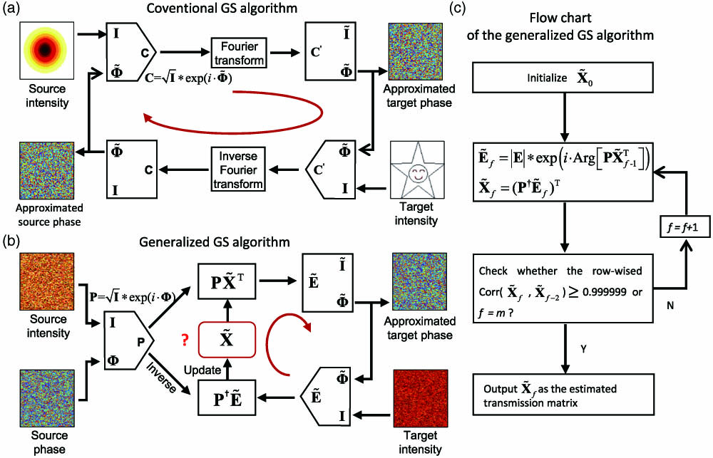
    Fig. 1. (a) Schematic view of the conventional GS algorithm to retrieve phase information from measured intensities. (b) Schematic view of the GGS algorithm to retrieve the propagating function (the optical TM). (c) The flowchart of the iteration process of the directly GGS algorithm. All parameters with approximated values are labeled with a tilde. The operator * indicates the element-wise multiplication between two vectors.
    Numerical evaluations of the GGS algorithm. (a) The statistical normalized enhancement as a function of γ=defL/N, when the TM is retrieved by the GGS 1 (black), GGS 2 (blue), and GGS 2-1 (red), respectively. Error bars: standard errors of 400 independent runs. (b) The correlations between |E|n and |E| measured in the target plane as a function of the adaptive parameter n. Error bars: standard errors of 200 independent runs when N=1000 and γ=4. (c) The statistical enhancement as a function of the number of independent control N, when retrieving the entire N×N TM at γ=4. Error bars: standard errors of N foci. (d) The histogram of the enhancement obtained from 1296 independent runs under different conditions. N=1296. The theoretical enhancement is denoted as the vertical dashed line.
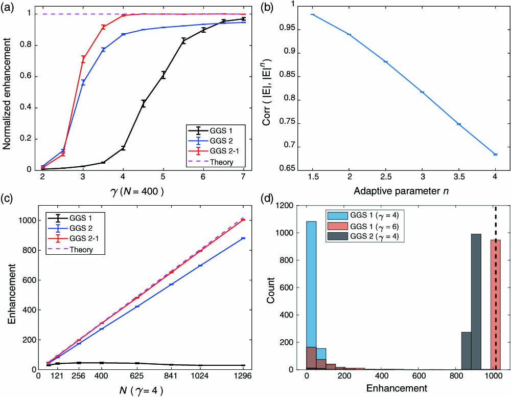
    Fig. 2. Numerical evaluations of the GGS algorithm. (a) The statistical normalized enhancement as a function of γ=defL/N, when the TM is retrieved by the GGS 1 (black), GGS 2 (blue), and GGS 2-1 (red), respectively. Error bars: standard errors of 400 independent runs. (b) The correlations between |E|n and |E| measured in the target plane as a function of the adaptive parameter n. Error bars: standard errors of 200 independent runs when N=1000 and γ=4. (c) The statistical enhancement as a function of the number of independent control N, when retrieving the entire N×N TM at γ=4. Error bars: standard errors of N foci. (d) The histogram of the enhancement obtained from 1296 independent runs under different conditions. N=1296. The theoretical enhancement is denoted as the vertical dashed line.
    Comparing the performance of different methods. (a) The achieved enhancement as a function of the number of independent control N when employing the GGS 2-1, EKF-MSSM, and prVBEM. γ=4 is fixed. Error bars: standard errors of 200 independent runs. (b) The computational time consumed for retrieving the entire TM. Except for the data denoted as the purple star being directly acquired from Ref. [20], the rest were computed using our computer and averaged from 200 independent runs. (c) The normalized enhancement (to the theoretical value, N=256 and γ=4) as a function of the SNR. Error bars: standard errors of 200 independent runs. (d) The absolute values of the correlation coefficients between one row of the correct TM and the retrieved TM when the probing fields are generated in a binary-amplitude format (N=64). Error bars: standard errors of 200 independent rows.
    Fig. 3. Comparing the performance of different methods. (a) The achieved enhancement as a function of the number of independent control N when employing the GGS 2-1, EKF-MSSM, and prVBEM. γ=4 is fixed. Error bars: standard errors of 200 independent runs. (b) The computational time consumed for retrieving the entire TM. Except for the data denoted as the purple star being directly acquired from Ref. [20], the rest were computed using our computer and averaged from 200 independent runs. (c) The normalized enhancement (to the theoretical value, N=256 and γ=4) as a function of the SNR. Error bars: standard errors of 200 independent runs. (d) The absolute values of the correlation coefficients between one row of the correct TM and the retrieved TM when the probing fields are generated in a binary-amplitude format (N=64). Error bars: standard errors of 200 independent rows.
    Experimental setup. BB1, BB2, beam block; BS, beam splitter; CCD, charge-coupled device; GG, ground glass; HWP, half-wave plate; L1, L2, lens; M, mirror; MMF, multimode fiber; OBJ1, OBJ2, objective lens; PBS, polarizing beam splitter; P, polarizer; SLM, spatial light modulator.
    Fig. 4. Experimental setup. BB1, BB2, beam block; BS, beam splitter; CCD, charge-coupled device; GG, ground glass; HWP, half-wave plate; L1, L2, lens; M, mirror; MMF, multimode fiber; OBJ1, OBJ2, objective lens; PBS, polarizing beam splitter; P, polarizer; SLM, spatial light modulator.
    Experimental demonstration of retrieving the TM of a stack of three ground glass diffusers. (a) The enhancement as a function of γ by using different methods. Error bars: standard error of 100 independent runs. (b)–(d) Camera-captured images of the formed 10 point foci, when the TM was retrieved from the same training data (the number of independent control N=720 and γ=4) with the GGS 2-1, GGS 2, and GGS 1, respectively.
    Fig. 5. Experimental demonstration of retrieving the TM of a stack of three ground glass diffusers. (a) The enhancement as a function of γ by using different methods. Error bars: standard error of 100 independent runs. (b)–(d) Camera-captured images of the formed 10 point foci, when the TM was retrieved from the same training data (the number of independent control N=720 and γ=4) with the GGS 2-1, GGS 2, and GGS 1, respectively.
    Experimental demonstration of retrieving the TM of an MMF. (a)–(c) Camera-captured images of the focus by conjugating one row of the retrieved TM with the GGS 1, GGS 2, and GGS 2-1 from the same training data set, achieving 82.4%, 71.5%, and 4.1% of the theoretical enhancement, respectively.
    Fig. 6. Experimental demonstration of retrieving the TM of an MMF. (a)–(c) Camera-captured images of the focus by conjugating one row of the retrieved TM with the GGS 1, GGS 2, and GGS 2-1 from the same training data set, achieving 82.4%, 71.5%, and 4.1% of the theoretical enhancement, respectively.
    Experimental demonstration of forming multiple foci through the MMF. (a)–(c) Camera-captured images of forming four foci simultaneously. With the GGS 2-1, the enhancements of A, B, C, and D reach about 64, 72, 77, and 89. With the GGS 2, the enhancements of A, B, C, and D reach about 49, 67, 57, and 66. Instead of forming four foci, the GGS 1 only generates C with an enhancement of 92. (d)–(f) Camera-captured images of forming five foci simultaneously. With the GGS 2-1, the enhancements of A, B, C, D, and E reach about 51, 64, 67, 74, and 82. With the GGS 2, the enhancements of A, B, C, D, and E reach about 49, 54, 50, 65, and 68. In contrast, the GGS 1 fails to function.
    Fig. 7. Experimental demonstration of forming multiple foci through the MMF. (a)–(c) Camera-captured images of forming four foci simultaneously. With the GGS 2-1, the enhancements of A, B, C, and D reach about 64, 72, 77, and 89. With the GGS 2, the enhancements of A, B, C, and D reach about 49, 67, 57, and 66. Instead of forming four foci, the GGS 1 only generates C with an enhancement of 92. (d)–(f) Camera-captured images of forming five foci simultaneously. With the GGS 2-1, the enhancements of A, B, C, D, and E reach about 51, 64, 67, 74, and 82. With the GGS 2, the enhancements of A, B, C, D, and E reach about 49, 54, 50, 65, and 68. In contrast, the GGS 1 fails to function.
    Guoqiang Huang, Daixuan Wu, Jiawei Luo, Liang Lu, Fan Li, Yuecheng Shen, Zhaohui Li. Generalizing the Gerchberg–Saxton algorithm for retrieving complex optical transmission matrices[J]. Photonics Research, 2021, 9(1): 34
    Download Citation