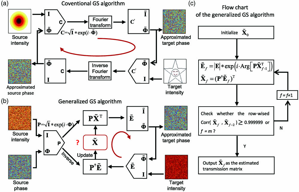
The fast oscillating nature of light prevents time-varying optical fields, especially the phase information, from being directly measured using optical detectors that generally provide the time-averaged intensity of light due to limited bandwidth. To retrieve the phase information, the holographic method is widely adopted, which beats down the fast oscillation by introducing a known reference field. Although it is widely adopted, introducing a reference field suffers from practical challenges in certain circumstances, such as wavefront sensing in astronomy and microscopy. Thus, retrieving field information from pure intensity measurements without using the holographic method is highly desired. In 1972, an iterative algorithm, namely, the Gerchberg–Saxton (GS) algorithm, was developed to retrieve the phase values from a pair of related intensity measurements [1]. This capability enables the GS algorithm, as well as other phase retrieval algorithms [2,3], to be widely used in many research areas including ultrafast signal processing, crystallography, ptychography, and holographic imaging [4–8]. Figure 1(a) illustrates the general scenario of the GS algorithm, where two planes, i.e., the source plane and the target plane, are related through a predefined propagating function. The mathematical form of this function is known and, for example, can be the Fourier transformation (realized through a lens in optics). In this relatively simple framework, the distributions of the source intensity and the target intensity are known, while the goal is to retrieve the phase distributions on these planes. Reference [1] proves that by initializing a random phase distribution on either of the planes and iterating along the loop (denoted as the red arrow), the approximate phase distributions on both planes will gradually converge to the correct ones.

Besides retrieving phase information on these planes, a remaining question is whether the GS algorithm can be generalized to retrieve the propagating function, if unknown, from the measured intensity. This question arises from the increasing need in biophotonics and optical communications to quantify the optical properties of complex media, such as a piece of biological tissue, a scattering wall, and a multimode fiber (MMF), for light focusing, imaging delivering, and recovering [9–15]. The optical transmission matrix (TM) of the complex medium is desired to be measured non-holographically as the propagating function.

Figure 1(b) describes the concept of generalizing the GS algorithm to retrieve the optical TM. The basic principle relies on the assumption of a linear system. For simplicity but without losing generality, the unknown TM of the complex medium is modeled as a matrix X with dimensions of M×N, which is encapsulated in a red box with a question mark. To probe the TM, a series of L random field patterns are generated in the source plane. During experiments, the probing field can be generated using a commercialized liquid-crystal-based spatial light modulator (SLM). For phase-only modulation, each element is generated with the same amplitude but randomly distributed phase values within a range of 0 to 2π. For mathematical convenience, all L field patterns can be grouped as a probing matrix P with dimensions of L×N: P=[eiθ1(1)⋯eiθN(1)⋮□⋮eiθ1(L)⋯eiθN(L)],(1)where N is the number of independent control segments of the SLM. The amplitude of each element was normalized to one for simplicity but could be replaced with physical values if needed. The subscript and the superscript denote the index of the elements in the source plane and the label of field patterns, respectively. After interacting with the complex medium, the resulting field in the target plane becomes E=PXT=[E1(1)⋯EM(1)⋮□⋮E1(L)⋯EM(L)],(2)where X is the to be determined optical TM (propagating function), and the operator T denotes matrix transposition. In practice, a detector array such as a camera is employed in the target plane to measure the amplitude distribution |E|. The number of pixels of the camera or the number of spatially independent intensity measurements sets the number of the rows M that can be retrieved for the TM. Like the conventional GS, we anticipate that by iterating along a certain loop (denoted as the red arrow), the approximated X˜, which is computed from P†E˜, converges to the correct X. Here, † denotes the operation of pseudo-inverse. The detailed operational procedure of the generalized GS (GGS) algorithm is illustrated in the flowchart of Fig. 1(c). At the beginning of the iteration, we generate the initial guess X˜0 for the TM. Then, the approximated field in the target plane at the fth iteration is constructed as E˜f=|E|*exp[i·Arg(PX˜f−1T)],(3)where * stands for element-wise multiplication, and Arg(·) computes the principal value of the argument of a complex number. This procedure is identical to the single-constraint situation in the error-reduction iteration algorithm [2]. The approximated TM is then updated as X˜f=(P†E˜f)T.(4)This iteration process terminates if the correlation between X˜f and X˜f−2 is larger than 99.9999% or the number of iterations reaches a preset value m. Unless specified otherwise, m is set to 1000 in this study. We note here that due to the periodic oscillating observed from the evolution of the numerical solution, the correlation is defined between X˜f and X˜f−2 rather than X˜f and X˜f−1. To save the computational resource, the correlation operation is performed row by row. Once a certain row in X˜ converges, this row is directly output as the final solution and will be removed from the rest of the iteration process. This operation gradually reduces the dimension of the matrix as the iteration proceeds, effectively mitigating the computational burden. Unlike the conventional GS algorithm, using the GGS algorithm to retrieve the optical TM is more like solving an overdetermined problem.

For optical TMs that are highly disordered, the directly GGS algorithm, namely the GGS 1, can be easily trapped into local optimums if the probing matrix is not large enough. We will show in the following that the GGS 1 requires at least 7N input field patterns and 7N camera-captured images to guarantee the accuracy of the retrieved TM. This value indicates that the GGS 1 needs more intensity measurements than other non-holographic methods reported in the literature (∼4N) [16,17]. To ease this problem, we introduce an adaptive parameter n in Eq. (3) as the power exponent to |E|. This operation is similar to artificial “heat data”, which is equivalent to increasing the entropy in the simulated annealing process [18]. We also tested adding random/Gaussian noises to make the data “chaotic”, but could not obtain significant improvement in terms of performance. In other words, |E|n is used to replace |E| when constructing the approximated field in the target plane. For naming purposes, the GGS 2-1 represents a two-step iteration process: n is chosen as two in the first step and decreases to one in the second step. In contrast, the GGS 1 or GGS 2 indicates that n is fixed at 1 or 2, respectively. This modification endows the GGS algorithm with the ability to jump out of local optimums. As a result, the required number of intensity measurements can be reduced to 4N for the GGS 2-1. Furthermore, compared with the previously developed non-holographic ones, including the extended Kalman filter with a modified speckle-correlation scattering matrix (EKF-MSSM) [16], the phase retrieval variational Bayes expectation maximum (prVBEM) [17,19,20], and semidefinite programming (SDP) [21,22], the GGS algorithm consumes much less computational resources in retrieving the huge TM, thus being orders of magnitude faster in terms of computational time.

We first evaluated the performance of the GGS algorithm numerically. Unless otherwise specified, all of the following simulation results were carried out through MATLAB2019a on a personal computer equipped with an i5-8600k 3.6 GHz CPU and a 16 GB RAM. No independent graphics card was employed to perform the auxiliary operation for large matrices. For complex media, the uncorrelated transmission coefficient (UTC) model was adopted to describe the TM, in which each element is drawn from a circular Gaussian distribution during simulations [23]. To quantify the accuracy of the retrieved TM, we followed the convention by sending in the conjugated field of a certain row in the TM, enabling the formation of an optical focus in the target plane [9]. The more accurate the retrieved TM is the better quality the focus has. In practice, the quality of the focus is quantified by the enhancement, which is defined as the intensity ratio of focus Ifoc and the ensemble-averaged speckles Iavg generated from a random input, i.e., η=Ifoc/Iavg [24]. For phase-only modulation, the theoretical enhancement is η=π(N−1)/4+1, where N is the column number of the TM and is also the number of independent controls of the system. We first investigated how the number of field patterns L generated in the source plan influences the performance of the GGS algorithm. For a fixed number of independent control N=400, Fig. 2(a) plots the enhancement as a function of γ=defL/N for three variants of the GGS algorithm, i.e., the GGS 1, GGS 2, and GGS 2-1. When γ=2, all three algorithms lead to enhancements that are far below the theoretical value, indicating the inaccurate determination of the TM. This situation is commonly seen in iteration-based error-reduction algorithms due to insufficient constraints. As γ gradually increases, the enhancements for all three cases increase accordingly. Statistically, GGS 2-1 performs best among the three cases, leading to enhancement reaching about 99.1% of the theoretical value at γ=4. In contrast, at γ=4, the GGS 2 and GGS 1 only achieve about 87.1% and 14.3% of the theoretical value, respectively. These results demonstrate the effectiveness of the introduced adaptive parameter n. When further increasing γ, an interesting observation is these two performance curves intercept near γ=6. Beyond this point, the GGS 1 surpasses the GGS 2. The validity of the introduced adaptive parameter n can also be understood in Fig. 2(b), where the correlations between |E|n and |E| are plotted. Even though the correlations between |E|n and |E| decay approximately linearly as n increases, high correlation always persists. This result also suggests that n=4, for example, can also be used as the initial value. In this work, we simply set n starts with two, as such a choice is good enough for the GGS algorithm to escape from local optimums.

After fixing γ=4, we also plotted the achieved enhancement as a function of N in Fig. 2(c). Specifically, at N=64, 121, 256, 400, 625, 841, 1024, and 1296, the enhancements achieved by the GGS 2-1 can reach 98.0%, 98.3%, 98.4%, 98.9%, 98.1%, 98.6%, 98.8%, and 98.6% of the theoretical value, respectively, indicating that the GGS 2-1 can always retrieve the TM with high accuracy. As a comparison, the enhancement achieved by the GGS 2 is slightly worse but can still achieve around 87% of the theoretical value. In contrast, the GGS 1, which is the directly GGS algorithm, exhibits much poorer performance than the other two. Moreover, being plotted as the black solid line, the enhancement achieved by the GGS 1 barely increases, even with the increased N, and stays around a low level of 30−45. This condition is because of being trapped into local optimums, and thus increasing the preset value m cannot help. To elucidate the situations of being trapped into local optimums, Fig. 2(d) shows the histograms of the enhancement obtained from different conditions when N=1296. For the GGS 1, it can easily get trapped into local optimums with very low enhancement when γ=4. This condition can be significantly improved by increasing γ to six. Although about 23% of the cases still lead to low enhancements, 76% of them can now produce enhancement close to the theoretical value. Further investigations on the GGS 1 reveal that when γ=7, 95% of the cases can converge to the global optimum, leading to enhancement close to the theoretical value (not shown in the figure). In contrast, for the GGS 2 at γ=4, although most of the cases are not trapped into local optimums, considerable errors still exist due to the incorrect choice of n at the end of the iterations. As a result, the achieved enhancements are a bit smaller than the theoretical value.

Next, we compared the performance of the GGS algorithm with other non-holographic methods reported in the literature in terms of accuracy, time, and robustness. Here, we mainly take three methods, i.e., the EKF-MSSM algorithm [16], the SDP algorithm [21,22], and the prVBEM algorithm [17,19,20], into consideration. Figure 3(a) plots the achieved enhancement using different methods as a function of N. The EKF-MSSM employs the extended Kalman filter to solve for nonlinear equations, exhibiting almost identical performance to the GGS 2-1 in terms of the accuracy of the retrieved TM. The prVBEM was originally developed in the binary format to be combined with a digital micromirror device (DMD). Nonetheless, it can be directly extended to the full-field version for a fair comparison without any difficulty. As shown in Fig. 3(a), the prVBEM (full-field version) works well only for small N. As N gradually increases, the achieved enhancement starts to deviate away from the other two, indicating its inappropriateness of handling a large TM. For the above three cases, the same training data set, including both the probing matrix and the measured intensity (4N), was used for a fair comparison. The SDP is not compared here, as it requires large computational resources and stops to function when N goes beyond 150 with our computer. We next compared the computational time consumed by each method to retrieve the entire TM. For simplicity, the TM is assumed to be a square matrix such that M(row)=N(column). As shown in Fig. 3(b), the SDP requires a larger γ (γ=lnN) and takes about 7.14×103s to retrieve the TM when N=100 (denoted as an orange star), thus being the most computationally expensive one. The computational time consumed by the EKF-MSSM and the prVBEM is represented by the blue and green dashed lines, respectively. Specifically, when the number of independent control N=1296 and γ=4, these two algorithms take about 9.3×105 and 2.1×104s to retrieve the entire TM. Even equipped with a high-performance computing facility, it was reported that the prVBEM algorithm still took about 4h/1.44×104s (denoted as a purple star) to retrieve a TM when N=1296 [20]. As a comparison, the GGS 2-1 took only 5.0×10−1 and 8.3×102s to retrieve the entire TM when N=121 and 1296, respectively, corresponding to 4.1×10−3 and 6.4×10−1s for one row. Figure 3(b) also shows that the computational time consumed by three variants of the GGS algorithm is on the same order, albeit the GGS 2 is the fastest at the cost of accuracy (roughly 12%). Moreover, although the GGS 2-1 needs one more step than the other two, it is found to consume less time than that consumed by the GGS 1. Such an observation can be attributed to the fact that the “2” step significantly facilitates the convergence process to the true solution. Therefore, the computational time consumed by the GGS algorithm is orders of magnitude shorter than that consumed by other non-holographic methods, indicating the superiority of the GGS algorithm in handling large matrices with many unknowns.

In practice, the existence of external noises will certainly deteriorate the performance of the GGS algorithm. For completeness, we investigated the robustness of the GGS algorithm, as well as other methods, under the influence of external noises. Figure 3(c) plots the normalized enhancement obtained with different methods as a function of the signal-to-noise ratio (SNR) when fixing N=256 and γ=4. The results associated with the SDP are not shown, as the SDP stops working for N>150 due to the shortage of computational memory when using the embedded cvx package [16]. During numerical simulations, the SNR is defined as the ratio between the measured averaged intensity and the standard deviation of the added Gaussian noise with a mean of zero. When the SNR is larger than 10, the GGS 2-1 and the EKF-MSSM exhibit similar performance and can well retrieve the TM. As the SNR becomes smaller than 10, all existing algorithms exhibit significantly degraded performance. An interesting observation is that although the GGS 2 performs slightly worse when the SNR is high, it is the most robust one in a noisy environment. It is worth noting that the existence of noises does not significantly affect the computational time consumed by the GGS algorithm. Another aspect to discuss is that in case of using fast SLMs like DMDs, the probing fields are generated in a binary-amplitude format [17,20,25–27]. In this condition, the GGS algorithm, as well as other methods, cannot retrieve the TM as accurately as before. To examine this difference, Fig. 3(d) plots the absolute value of the correlation coefficients between the retrieved TM and the correct TM. As seen from the figure, the correlation coefficients stay around a constant level of 0.6, regardless of γ and the methods. Coefficients less than one result in downgraded performance, which could be solved by introducing additional constraints and will not be discussed here. Nonetheless, a correlation of 0.6 is still acceptable for many applications.

Having numerically evaluated the performance of the GGS algorithm, we built an experimental setup to retrieve the TM of complex media for demonstration purposes. The schematics of the setup are shown in Fig. 4. A continuous-wave laser (MDL-C-642-30mW, CNI), operating at 642 nm wavelength, was used as the light source. Before illuminating the SLM (PLUTO-2-NIR-011, Holoeye, 1920×1080 pixels, 8 μm/pixel), the beam was expanded by a pair of lenses L1 and L2 to 1 in. (2.54 cm). The modulated light was then directed to the complex medium, whose TM needs to be retrieved. During experiments, the randomly generated input wavefront was sent to probe the complex medium, and the resulting output intensity patterns were measured using an 8 bit CCD (GS3-U3-32S4C, Point Grey). The measurement SNR during the experiment was quantified to be around 25.

To reproduce the simulation results presented in Fig. 2(a), we first chose a stack of three ground glass diffusers (DG10-120, Thorlabs) as the complex medium. By fixing N=90, Fig. 5(a) plots the averaged enhancement as a function of γ by using different methods. Specifically, for the GGS 2-1, the experimentally achieved enhancements reached 5.4%, 33.75%, 55.7%, 59.4%, 59.8%, and 60.9% of their corresponding theoretical value when γ=2, 3, 4, 5, 6, and 7, respectively. As expected, the red curve becomes flattened after γ becomes larger than 4, which agrees with the observation that the enhancement saturates at γ=4 in Fig. 2(a). The slight increase in the enhancement after γ=4 is due to the nonzero measurement noise during experiments. Compared to the GGS 2-1, the enhancement achieved by the GGS 2 has a similar trend but slightly worse performance. Same for the simulation results, the experimentally achieved enhancement by the GGS 1 is even smaller, confirming that the directly GGS algorithm can be easily trapped into local optimums. These results demonstrate the advantages of introducing an adaptive parameter n in the GGS algorithm. Results obtained by using the EKF-MSSM and prVBEM are also presented, exhibiting similar performance to the GGS 2-1 in terms of accuracy when γ≥4. It is worth noting that since prVBEM adopts a statistical estimation method, it demonstrates the best performance among the three when γ is small. With the retrieved TM, any patterns can be synthesized on the target plane. As typical examples, Figs. 5(b)–5(d) show the camera-captured images, synthesized by using 10 rows of the retrieved TM (γ=4 and N=720) using the GGS 1, GGS 2, and GGS 2-1, respectively. Among all three cases, these foci achieved with the GGS 2-1 are the brightest [Fig. 5(b)], with the averaged enhancement of the 10 spots reaching 65.6% of the theoretical value. Here, the theoretical value of the enhancement should be modified by inserting an additional Nf in the denominator, where Nf is the total number of foci in the target plane. As a comparison, the foci achieved with the GGS 2 are slightly dimmer [Fig. 5(c)], with the averaged enhancement reaching 62.5% of the theoretical value. Moreover, the GGS 1 fails forming the desired pattern as being trapped into local optimums, leading to speckles in the captured image [Fig. 5(d)].

We further demonstrated retrieving the TM of a 1-m-long MMF. The step-index MMF is silica-based (refractive index∼1.48) with a core diameter of 50±2.5μm and a numerical aperture of 0.200±0.01 (FC/PC-FC/PC-50/125–900 μm–1 m, Shenzhen Optics-Forest Inc.), thereby supporting about 1200 modes at 642 nm. Figure 6 shows the camera-captured images, formed by conjugating one row of the TM retrieved (γ=4 and N=400) using the GGS 2-1, GGS 2, and GGS 1, respectively. Among all three cases, the focus achieved with the GGS 2-1 is the brightest, with the enhancement reaching 76% of the theoretical value. The focus achieved with the GGS 2 is slightly dimmer, with the enhancement reaching 67% of the theoretical value. The focus achieved with the GGS 1 has an enhancement that reaches only 5% of the theoretical value, leading to observable speckles in the background.

Synthesizing multiple foci on the target plane was also demonstrated through the MMF. Figures 7(a)–7(c) show the camera-captured images of simultaneously focusing light to four separated spots, when the TM was retrieved (γ=4 and N=600) using the GGS 2-1, GGS 2, and GGS 1, respectively. In Fig. 7(a), the enhancements of the four foci labeled with A, B, C, and D are 64, 72, 77, and 89, respectively. The averaged enhancement reaches 64% of the theoretical value. The TM retrieved using the GGS 2 also allows simultaneously focusing light to the same four spots, with averaged enhancement reaching 51% of the theoretical value. However, by using the TM retrieved with the GGS 1, multi-spot focusing cannot be achieved. Instead, only one focus was realized and can be observed. We further demonstrated simultaneously focusing light on five spots, with camera-captured images shown in Figs. 7(d)–7(f). Again, with the TM retrieved by using the GGS 2-1, five bright foci, labeled with A, B, C, D, and E, achieve the enhancements of 51, 64, 67, 74, and 82, respectively. The averaged enhancement of these five foci reaches 72% of the theoretical value. Similarly, the TM retrieved using the GGS 2 allows multi-spot focusing, with averaged enhancement reaching 61% of the theoretical value. By using the TM retrieved with the GGS 1, multi-spot focusing cannot be achieved. These experimental results demonstrate the superiority of the GGS 2-1 in retrieving the optical TM of arbitrary complex media.

Notably, the experimentally obtained enhancements are always below the theoretical value. This observation is not originated from the algorithm, but is due to practical reasons including the inaccurate phase values of the SLM, intensity fluctuations of the laser, detection noise of the camera, and time-varying characteristics of the complex media. Nonetheless, optical foci with enhancements reaching 60%−70% of the theoretical value are still among the highest performance. Moreover, the computational time cost by the GGS algorithm can be further optimized. The current termination rule of the GGS algorithm is either that the correlation coefficients between two iterations X˜f and X˜f−2 are larger than 99.9999% or the number of iterations reaches the preset maximum value m=1000. In most cases, we found that the GGS algorithm rapidly converges before m reaches 1000, and the correlation coefficients reaching 99.9999% as the termination rule is appropriate. Taking the GGS 2-1 as an example, when generating the data point at N=1296 in Fig. 2(c), the two steps with different adaptive parameter n on average take around 287 and 34 iterations, respectively. By relaxing the criteria to 99.999%, these two values decrease to around 190 and 23 at the cost of 0.1% accuracy, thereby reducing the computational process without significantly sacrificing the accuracy of the retrieved TM. Similarly, by setting the criterion to 99.9999%, these two values increase to around 296 and 46 but the accuracy remains unchanged, indicating that 99.9999% is a good choice. We could also investigate more on the choice of the adaptive parameter n in future works to facilitate the convergence rate of the GGS algorithm by varying the initial value and the decay trend. As a final remark, as N increases, the number of steps consumed before converging will also increase. Therefore, we may enlarge m for a larger N.

In summary, we generalized the GS algorithm to retrieve the unknown propagating function, i.e., the optical TMs of complex media, from intensity measurements on the target plane. An adaptive parameter n in the power exponent of the intensity constraint (|E|n) was introduced to facilitate the computational process. We numerically showed that the GGS 2-1 can accurately retrieve the TM when γ=4. With the same training data set, the computational time cost by the GGS 2-1 is orders of magnitude shorter than other reported non-holographic methods in the literature. This feature is highly desirable in handling a large TM. The performance of the GGS algorithm was further demonstrated by retrieving the optical TM of a stack of three ground glass diffusers and an MMF, enabling arbitrary patterns (single and multiple foci) to be projected through these media. Quantitatively, enhancements around 60%−70% of the corresponding theoretical values can be routinely achieved for these foci, indicating the accuracy of the retrieved TM using the GGS algorithm. Due to its superior performance and the relatively simple computational framework, the GGS algorithm is promising to become a powerful tool in fast retrieval of a large optical TM of complex media from pure intensity measurements, allowing a broad range of applications in biomedical optics and optical communications.

References

[1] R. W. Gerchberg. A practical algorithm for the determination of phase from image and diffraction plane pictures. Optik, 35, 237-246(1972).