Land surface temperature (LST) affects numerous climatological, meteorological, ecological, and geophysical phenomena, which in turn affect the LST. As one of the key parameters for land surface process studies at global and regional scales, LST plays a vital role in processes such as surface water and energy exchange (Sellers, 1988). Therefore, accurate determination of LST is valuable for global climate change research, disaster monitoring, and resource management (Ma and Ma, 2006; Wu et al., 2005).

Currently, the study of LST is limited by observation conditions: ground-based observation sites have sparse spatial distributions and low temporal frequencies; stationary meteorological satellites’ products have low spatial resolutions (generally 3 to 5 km); polar-orbit satellites’ products possess high spatial resolutions (generally 1 km), however, it is difficult to obtain temporal and spatial continually land surface process information by only using polar-orbit satellites’ observations. This limitation is mainly because the observation times at the same site are irregular. What’s more, the limitations in inversion algorithm cause an overall bias in the LST. Although the land surface model relies on its intrinsic physical processes and dynamic mechanisms, land surface variables of continuous evolution in time and space can be obtained; however, due to the uncertainties of physical and dynamic mechanisms and parametric schemes, the accuracies of existing global and regional climate models and land surface models have yet to be improved.

In view of coping with the shortcomings of LST observations and land surface model simulations, a land surface data assimilation technique that combines temporally discontinuous observation data with a land surface model that is continuous in space and time has become an effective method for obtaining high-quality LST data. Current domestic and foreign major land surface assimilation systems mostly include the assimilation of variables such as atmospheric driving data and soil moisture (Rodell et al., 2004; Mitchell et al., 2004; Xia et al., 2012; Zou et al., 2006; Balsamo et al., 2007; Lim et al., 2006; Shi et al., 2011; Han et al., 2017; Shi et al., 2014), and there is little research on the assimilation of LSTs. Existing LST assimilation studies mainly focus on improvements to the assimilation scheme. Variational Assimilation Algorithms have been used to assimilate LSTs via the common land model (CoLM) (Meng, 2012), where the assimilation constraint conditions used were surface and vegetation energy balance equations in the CoLM model, and the adjustment factors were the bare soil and vegetation evaporation ratios. The results showed that the assimilated LST and evapotranspiration results were closer to the measured values ​​at Bonville Station via the AmeriFlux network. A local ensemble transform-based Kalman filter (LET-KF) analysis for LST sequences based on the complementary prediction of transient models was proposed to solve the problem of the low prediction accuracy of traditional LST sequence analysis methods (Wang, 2016); the verification results showed that the algorithm effectively improved the accuracy of the LST predictions. To improve the temporal resolution and accuracy of LST observations, the assimilation method has been used to downscale Meteosat LSTs under non-uniform surface conditions (Mechri et al., 2016); the results, compared with those of the original model, show that the deviation and root mean square error (RMSE) are reduced. Some studies have applied new observational data to the assimilation system, which improves the simulation effect of LST. Based on the ensemble Kalman filter (EnKF), LST data derived from the new generation of Chinese meteorology satellites (FY3A-VIRR) are assimilated into the CoLM for the first time (Xu et al., 2015). The results show that the dual-pass data assimilation scheme can reduce the model uncertainty and improve the prediction of surface energy fluxes. A one-dimensional land data assimilation scheme based on the EnKF and CoLM version 3.0 has been developed (Huang and Liu, 2015) to assimilate the Moderate Resolution Imaging Spectroradiometer (MODIS) leaf area index (LAI) and LST; the results show that LST assimilation improves the simulation of soil temperature profiles.

LST is directly affected by shortwave solar radiation and has strong temporal and spatial variations (specifically distinct diurnal variations). During the assimilation of LST data, the diurnal variations in LST observations undoubtedly affect the accuracy of the assimilation results. Properly using temporal information from satellite observations during the assimilation process and enabling the results of the LST assimilation to be more accurate are problems that must be solved during the process of data assimilation when using satellite observation data. Therefore, not considering diurnal variations in LST during assimilation may have a significant effect on the assimilation results of LST. However, few studies have focused on the effects of diurnal variations in LST during the assimilation process.

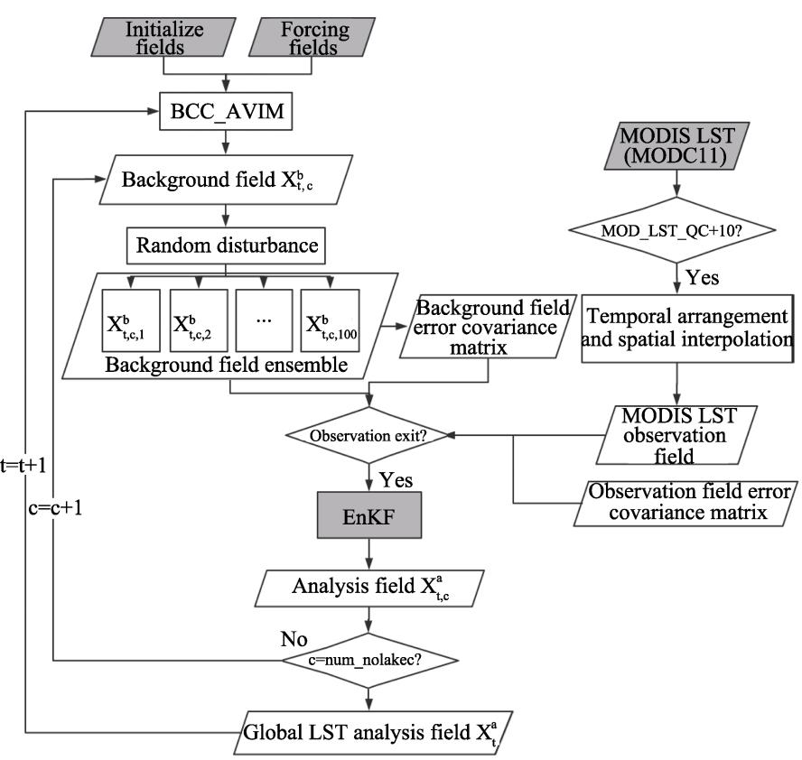
Based on the Beijing Climate Center Atmosphere-Vegetation Interaction Model (BCC_AVIM), this article uses the EnKF algorithm to assimilate the global MODIS LST product and focus on how diurnal variations in LST observations impact assimilation. The assimilation data of each experiment are observation data containing different diurnal variations for LST. The LST product of Global Land Data Assimilation System (GLDAS) was used to verify the simulation results of each experiment and analyse the impact of diurnal variations in LST on the assimilation results.

The land surface model is a numerical model describing matter and energy exchange in land surface and soil and is a significant component of the climate system model. The BCC_ AVIM land surface model (Wu et al., 2014) used in this paper was developed based on Community Land Model (CLM) Version 3.0 (Oleson, 2018) and Atmosphere-Vegetation Interaction Model Version 2.0 (Ji et al., 2008). BCC_AVIM, as the land surface component of the Beijing Climate Center Climate System Model (BCC_CSM), has been used in the Coupled Model Intercomparison Project Phase 5 (CMIP5) experiment and has a certain ability to simulate the land surface carbon cycle and terrestrial ecosystem in the 20th century (Wu et al., 2013).

In the BCC_AVIM, the formula that calculates the LST at the n+1 time step using surface temperature at the n time step is shown in formula (1):

where T_g, S⃗g,L⃗g, H_g, E_g, and G respectively represent the surface temperature, net shortwave radiation, net longwave radiation, sensible heat flux, water vapour flux (kgm^-2s^-1) and surface heat flux. The variable λ represents the thermal conductivity (Wm^-1K^-1), ε_g=0.97 represents the lake reflectivity, σ is the Stefan-Boltzmann constant (Wm^-2K^-4), ρ_atm represents the moist air density (kgm^-3), C_p represents the air specific heat capacity (Jkg^-1K^-1), r_ah represents the sensible aerodynamic drag (sm^-1), r_aw represents the water vapour transport aerodynamic resistance (sm^-1), qsatTgrepresents the saturated humidity (kgkg^-1), λ₁ represents the first layer soil thermal conductivity (Wm^-1K^-1), and Δz₁ represents the soil thickness of the first layer (m).

The above formula indicates that LST is calculated from the radiation flux, surface gas flux, and surface status variables in the BCC_AVIM land surface model, and LST is directly involved in the calculation of related parameters for soil temperature and soil moisture (Oleson, 2018), Therefore, accurately simulating the LST is helpful for increasing the model accuracy when simulating other variables, such as soil temperature and soil moisture.

Evensen (1994) proposed the EnKF algorithm (Evensen, 1994). The EnKF has been used in the Lorenz system, which proved that the EnKF algorithm can obtain phase-space conversion information (Evensen, 1997). The EnKF method uses a dynamic sample ensemble that changes with time to represent the background error covariance matrix (Burgers et al., 1998). The size of the sample ensemble is generally 10-100. The number of samples (N) in this experiment is set to 100.

Suppose that x^b represents the m-dimensional background field, x^o represents the p-dimensional observation field, and H represents the observation operator, which is used to interpolate the model space in observation space. P^b Represents the m×m observation error covariance. In the matrix, R represents the observation error covariance matrix p×p. The minimum error covariance of the analytical field x^a is estimated by the following formula:

where K represents the Kalman gain or Kalman weight, which represents the weights of the background and observation fields during the analysis field calculations. Interpolating the weights (K) for all grid points via the (x^o-Hx^b) term updates the model results. The output of the model depends on the calculation of the background error covariance P^b:

where N represents the number of samples in the ensemble and A′ represents the m×N set perturbation matrix, which is defined as:

where xibrepresents the i-th ensemble member in the background field ensemble sample, and Ābrepresents the average of samples in the ensemble. When performing an assimilation algorithm, each background field ensemble member is compared with the observations, and the model results are updated according to formula (2).

Figure 1 shows the cycle of the assimilation scheme used in this study. The observation data are assimilated into the BCC_AVIM model circularly by each column and time. The cycle of the assimilation scheme begins with 100 samples generated by the historical integration of the land surface model. Combined with the observation data, the assimilation experiment is performed through the EnKF algorithm to obtain the analysis field at time t. Then, this analysis field is used as the initial field of the model at time t+1 to participate in the assimilation process. The continuous cycle of the assimilation can be carried out.

Land surface models need atmospheric variables to drive the model when calculating sensible heat, latent heat, and other ground fluxes, and most of the atmospheric driving data used in land surface models are derived from reanalysis data (Deng et al., 2010). The BCC_AVIM land surface model uses the National Centers for Environmental Prediction (NCEP) atmospheric reanalysis data as the forcing data; the NCEP atmospheric reanalysis data uses a T62L28 grid, with a horizontal resolution of 2.5°×2.5°, and the assimilation scheme is a three-dimensional variational assimilation (3D-Var). The variables included in the atmospheric forcing data are 2-m ground temperature, 10-m wind speed, relative humidity, precipitation rate, downward shortwave radiation, and atmospheric pressure. These required variables have been interpolated on the T106 grid, with a horizontal resolution of 1.125°×1.125° and a temporal resolution of 3 hours.

MODIS, which is mounted on the Terra/Aqua satellites, is an instrument used to observe global biological and physical processes in the Earth Observing System (EOS) programme (Wan and Li, 1997). It has 36 mutually matched spectral bands. The spatial resolution of a point under the satellites can be 250 m, 500 m, and 1000 m, with a field-of-view width of 2330 km. MODIS can obtain images of land and ocean temperatures, primary productivity, land surface coverage, clouds, aerosols, vapours and fires. The LST obtained by the MODIS observations is mainly dependent on the split window algorithm in the remote sensing inversion method. It is calculated by using the 31st and 32nd MODIS bright temperature channels, atmospheric transmissivity, and surface illumination. MODIS has a total of 7 surface temperature products (Wan, 2009), which are MOD11_L2, MOD11A1, MOD11B1, MOD11A2, MOD11C1, MOD11C2, and MOD11C3. Among them, C1, C2, and C3 are all global gridded products, with a spatial resolution of 0.05°. The difference between them is the difference in the temporal resolution. The C1 product is produced by the splicing and re-sampling of the B1 product, with a temporal resolution of 1 day. The C2 product is obtained by simply averaging the data of the C1 product over 8 days. The C3 product is obtained by simply averaging the data of the C1 product over one month. In this paper, the global gridded data of the MOD11C1 product with the highest temporal resolution is selected as the LST observation data for assimilation.

MOD11C1 product data for two years (from January 2014 to December 2015) are used in this study, with a spatial resolution of 0.05°×0.05°. These data include variables such as LST (day/night per hemisphere) and observation time (day/night per hemisphere), as shown in Figure 2. Selecting grid points starting with a “10” in the quality control (QC) flag indicates that the average error is less than 3 K; therefore, good quality data can be obtained. According to the temporal information of the grid, the daytime and nighttime LST in each hemisphere are processed at different time intervals, and the daytime and nighttime observations at the same time are stitched together and interpolated on a grid of 0.25°×0.25° using the average area interpolation method. Taking June 1st, 2014, as an example, Figure 3 shows the results of the MODIS surface observation data after preprocessing. (a) Through (d) show the 0 to 3 UTC, 0 to 6 UTC, 0 to 12 UTC, and 0 to 24 UTC LST observation data distributions, respectively. From Figure 3, we can see that the longer the observation interval is, the more observation information is contained; when the observation time interval is 24 hours, the daily mean surface temperature of the global grid points can be obtained.

The GLDAS was developed by the NASA Goddard Space Flight Center (GSFC) and the National Oceanic and Atmospheric Administration (NOAA) NCEP (Houser, 2004). The GLDAS uses the data provided by a new generation of ground-based and satellite observation systems to constrain the simulated land surface state. It is composed of a set of global high-resolution, off-line (i.e., separate from the atmosphere) land surface model systems containing satellite and ground-based observation variables to produce the best surface state and flux field in near real time. GLDAS data are often used as test data for new model and assimilation system abilities. Advanced Microwave Scanning Radiometer-Earth Observing System (AMSR-EOS) data have been used to analyse the reliability of GLDAS-simulated LSTs for one year, and the results showed that the GLDAS LST data are more reliable than the soil moisture data (Fu and Wang, 2014). Currently, the GLDAS includes three land surface models: mosaic, Noah and CLM. This article compares and evaluates the output of the land surface model by using the CLM for a global 3-hour LST product (with a horizontal resolution of 1°×1°).

To study the implication of diurnal variation information in LST observation data to assimilation, satellite observation data were processed at different time intervals, and the processed observation data were subjected to the assimilation experiment using the EnKF algorithm. The BCC_AVIM model simulation result was used as the control experiment (CTL). The experimental design is shown in Table 1. The first three years were used as the model spin-up time; after spin-up, four groups of satellite observation data at four different time intervals were used for assimilation for two years. The time step of the model was set to 30 minutes. At each time step, only the grid points that had observation data were assimilated, and the grid points without observations remained unchanged. It can be seen from Figure 2 that a grid point sometimes has two observations in one day, during the daytime and nighttime, respectively. In ASSI4, the data assimilated into the model were the average of the two values in one day. In ASSI3 and ASSI2, at each time step, only the grid points that have observation data at that time were assimilated. In ASSI1, no more than two time periods had observation data for a same grid point; therefore, the grid point was only assimilated within these two 3-hour periods and was not assimilated for the rest of the period. The experimental results were output on a daily basis, indicating the daily average status after assimilating the observation data; then, the results were compared with the GLDAS to obtain the relative accuracy of different assimilation experiments.

Since the GLDAS data are on a global grid, the time series is complete and, to some extent, the series can reflect the real changes in the LST; therefore, we use the GLDAS to quantitatively evaluate the results of each experiment. Using the bilinear interpolation method, the GLDAS is interpolated over the T106 grid, and the horizontal resolution is 1.125°×1.125°, which matches that of the observation data and model output. The bias, RMSE and correlation coefficient of the experimental results, combined with the GLDAS values of the individual grids, are calculated separately. Grids with missing values have not been included in the comparison. Three indicators (bias, RMSE, and correlation coefficient) were used to test the results. The calculation formulas of these three indicators are as follows:

where N represents the length of time, and A_i and B_i represent the experimental results and the GLDAS LST values at time i, respectively.

The surface temperature is directly affected by shortwave solar radiation and, thus, has obvious diurnal variations. Taking the global mean temperature in January and July 2014 as an example, the LST has been processed at different time intervals. The time series of the globally averaged LST is shown in Figure 4. It can be seen that the longer the time interval of the observations is, the weaker the diurnal variation in the LST contained in the sequence. In the observation sequence at the 24-hour interval, no diurnal variation information was included in the sequence; in the observation sequence at the 12-hour interval, the sequence contained significant day-night cyclical changes. In the observation sequence at the 6-hour interval, periodic oscillations in the diurnal variations in LST became more intense. In the observation sequence at the 3-hour interval, the number of grids that had observations at each time interval was small, and there were geographical differences; therefore, it showed a larger amplitude oscillation.

Taking the GLDAS LST as a reference, the experimental results were analysed using the three indicators of absolute bias, RMSE, and correlation coefficient. Table 2 compares these three indicators among the five groups of experiments, and it can be seen that the absolute deviation and RMSE are the smallest in the ASSI2 experiment, the largest correlation coefficient occurs in the ASSI1 experiment and the correlation coefficients for ASSI2 and ASSI1 are similar. From the comparison, we can see that the results of the assimilation using observations at 6-hour intervals are closest to the GLDAS LST.

Next, using the three indicators of bias, RMSE, and correlation coefficient, the impacts of diurnal variations in LST on the assimilation results were analysed in time and space.

3.2.1 Bias

This chapter uses the bias index to compare the experimental results with GLDAS LSTs. It can be seen in Figure 5 that compared with those of the CTL experiment, the bias values for the four groups of assimilation experiments are all reduced; in the CTL experiment, the large negative bias values over North Africa and South America and the large positive bias values over Oceania and the high-latitude regions of the Northern Hemisphere have all decreased in the assimilation experiments. By combining the average absolute bias in Table 2, it can be seen that the global average bias decreases most when using 6-hour interval observations to perform the assimilation.

One of the characteristics of polar-orbit satellite observations is that each grid point corresponds to a different observation time. According to the temporal information for each grid point, daily observation data are divided into equal time period intervals. For observation data with different time intervals, when the observation time interval is shorter, the observation data entered into each assimilation window are more accurately related to the corresponding time period. The bias of the ASSI2 experiment is less than that of the ASSI1 experiment because the observation time interval of the ASSI2 experiment is longer; under the premise that diurnal variations are taken into consideration, the more observation information that is assimilated for each time step in the model, the better the assimilation results. When assimilating the 24-hour interval data, the amount of observation information is greater, but the assimilation effects are worse because the daily mean value ignores the diurnal variation information; therefore, related to this time period, the deviation in the observation time is large, and the overall error is large due to the accumulation in the assimilation window. Therefore, in the ASSI4 experiment, the observations of the global grid points can be assimilated via the model at each time, but the bias values of the results are greater than those of any other assimilation experiment.

Due to the differences among the assimilation effects in different regions, the land grids were divided into plates based on the distribution of continents, and the bias for each grid point was counted, as shown in Figure 6. As a whole, the bias values of the assimilation experimental results globally and for each plate are more symmetrical than those of the CTL experiment, and the number of grid points with large and minimum bias values decreases. It can be seen that the BCC_AVIM LST simulation results are lower than the GLDAS LSTs in most areas, and the assimilation experiments have improved the simulation results by adding the assimilated MODIS LST observations. The ASSI1 and ASSI2 experiments have the best results; most grid point deviations are limited to ± 2 K. In the ASSI3 and ASSI4 experiments, the number of negative bias grids has decreased significantly, but the number of positive bias grids has increased. This result is related to the fact that MODIS observations are higher than GLDAS LSTs.

According to Figure 5, in the CTL experiment, the LST of the Eurasian continental plate (1°17′N-77°43′N, 9°31′W-180°E) is higher in mid- to high-latitude areas and lower in low-latitude areas. In Figure 6, there are more grid points with large positive and negative biases via the CTL experiment, and they are distributed symmetrically along the zero line. The positive and negative bias grids over the Eurasian continental plate are reduced in the assimilated experimental results, and all assimilation experiments have similar effects (mean bias of four experiment in Eurasia < 1K), indicating that for the Eurasian continental plate, the effects of assimilation using observations at different time intervals vary less; therefore, whether or not to consider diurnal variation information has little effect on the results of assimilation.

According to Figure 5, the LST of the African continental plate (34°51′S-37°21′N, 17°33′W-51°24′E) is mainly low. From the analysis shown in Figure 6, the longer the observation time interval is, the more observation information is assimilated into the model, and more negative bias grids change into positive bias grids. The number of positive biases in the ASSI3 (1.28K) and ASSI4 (1.62K) experiments is greater than the number of negative bias grids, indicating overcorrection features. For the African continental plate, the best results were derived from the ASSI1 (0.14K) and ASSI2 (0.28K) experiments (i.e., the experiments that take into account the LST diurnal variation information).

The Oceania continental plate (47°S-30°N, 110°E-130°E) results are similar to those of the African continental plate. The number of positive biases in the ASSI3 (1.20K) and ASSI4 (1.44K) experiments is greater than the number of negative bias grids, while the best results were derived from the ASSI1 (-0.02K) and ASSI2 (0.12K) experiments. The diurnal variation information of LSTs when assimilating can improve the results.

Figure 7 shows the time series of the bias values for all experiments. To better compare the results, the bias value for each grid point is taken as an absolute value, and the absolute bias is calculated. It can be seen that the absolute bias values for all of the assimilation experiments are reduced compared with those from the CTL experiment, except for those in individual months. From Table 2, the average absolute bias of the ASSI2 experiment is the smallest. It can be seen from Table 3 that in different months, the experiment with the smallest absolute bias varies, and the minimum absolute bias appears mainly in the ASSI2 experiment. In March, April and July of 2014 and March, April and July of 2015, the minimum absolute bias occurred in the ASSI4 experiment. The reason is that in the ASSI4 experiment during these months, the absolute bias values over Africa and Oceania are greater than those in the ASSI2 experiment, but the absolute bias values over Eurasia, North America, and South America are less than those via the ASSI2 experiment. In most cases, to increase the accuracy of the observation information relative to the time of the corresponding assimilation window during assimilation, observations with shorter intervals are used for assimilation (i.e., by considering the diurnal variation information of the observations), and better assimilation results can be obtained. However, in some months (e.g., March and April) and in some areas where the diurnal variations in LST are small, the observation interval can be appropriately bigger; this way, the assimilation effect can improve by increasing the number of observations at a single time.

3.2.2 RMSE

Biases can represent the positive and negative differences between simulated values and true values, while the RMSE is more sensitive to the extreme value in a group of numbers and can reflect the discrete degree of the simulated effect. This section uses the RMSE to analyse the experimental results from 2014 to 2015 from a time and space perspective.

From Table 2, we know that the average global RMSE of assimilation experiments ASSI1-ASSI3 is lower than that of the CTL experiment, but that of the ASSI4 is higher. Similar with the bias analysis results, the RMSE analysis results are better in the ASSI2 experiment than those in the other experiments. Different observation time intervals have different effects on different regions. For the Eurasian continent, the RMSE is smaller when the 6-hour interval observations are used for assimilation; for the African continent, when the 3-hour interval observations are assimilated, a smaller RMSE can be obtained. Without considering diurnal variations in LST observations will increase the dispersion of the simulation results, which has a bad influence on the assimilation results. At smaller time intervals, diurnal variations in the LST are preserved. To reduce the RMSE of the simulation results and the temporal dispersion of areas with large diurnal variations in LST, the same assimilation window should be used to enter the observation information more accurately relative to the time of observation.

Figure 9 shows the RMSE of the simulated LST and GLDAS LST for the CTL and assimilation experiments over time. The RMSEs of the CTL and assimilation experiments are smaller in northern summers and larger in northern winters. The RMSEs for each month in the ASSI1 and ASSI2 experiments are smaller than that in the CTL experiment. The ASSI3 experiment RMSE is smaller than that of the CTL experiment (except for June 2015). The ASSI4 experiment RMSE is smaller than that of the CTL experiment in northern winters (December, January and February), and the remaining RMSEs are larger than in the CTL experiment. The average RMSEs of the CTL and four assimilation experiments are shown in Table 2. It can be seen from Table 4 that on representative months, the ASSI2 experiment has the smallest RMSE. Through the analysis of time and space, it is known that by taking into account observed diurnal variation information, the RMSE of the assimilation results can be reduced.

3.2.3 Correlation coefficient

The correlation coefficient is an indicator that studies the degree of linear correlation between two variables. By using the correlation coefficient to evaluate the experimental results, the degree of similarity between the simulation and true value results at each grid point

can be obtained. As shown in Figure 10, in the CTL experiment, the correlation coefficients

over central Africa and northern South America are relatively small. The correlation coefficients for the above areas during the four assimilation experiments all increased. The correlation coefficients at mid- to high latitudes in the Northern Hemisphere and over the continent of Oceania in ASSI1 and ASSI2 all improved, while those in ASSI3 and ASSI4 did not improve much. Overall, the ASSI2 experimental results are more relevant to the GLDAS LST data.

Figure 11 shows the changes over time in the correlation coefficient between the simulated LSTs in the CTL and assimilation experiments and the GLDAS LSTs. It also can beseen from Table 5 that the correlation coefficient between the ASSI1 experimental results and the GLDAS LST is greater than that with the CTL experiment, and the correlation coefficient between the ASSI4 experimental results and the GLDAS LST is relatively small. The average correlation coefficients of the CTL and assimilation experiments are shown in Table 2. The ASSI1 experiment has the largest correlation coefficient of the assimilation experiments, followed by ASSI2 and ASSI3. These results show that processing satellite data into 3-hour time intervals and taking into account diurnal variations in LST when assimilating observation data can yield results that are more similar to changes in GLDAS LST.

Based on the BCC_AVIM land surface model, this paper uses the EnKF algorithm to assimilate the MODIS LST product. Different experiments have been designed to assimilate observation data with different time intervals, and the GLDAS LST product is used to verify the experimental results. The assessment was conducted to analyse the effects of diurnal variations in LSTs from satellite observations on LST assimilation results with a land surface model. The main conclusions are as follows.

(1) The LST is directly affected by shortwave solar radiation and, thus, has distinct diurnal variations. For polar-orbit satellite observations, the longer the time interval is, the weaker the diurnal variation in the LST contained in the sequence. When the observation time interval is 24 hours, no diurnal variation information is included in the sequence; when the observation time interval is 12 hours, the sequence contains significant cyclical changes in the LST. When the observation time interval is 6 hours, the diurnal variations in the LST oscillations are more intense; when the observation time interval is 3 hours, the number of observations contained in each time period is small, and there are regional differences. Therefore, it is easy to show large oscillations.

(2) The BCC_AVIM global LST simulation results are lower than those of the GLDAS LST, with large negative biases over North Africa, South America, and Oceania and large positive deviations at high latitudes in the Northern Hemisphere. After assimilating the MODIS LST observations, the extremely positive and negative bias values were reduced, and the model's ability to simulate LST improved both globally and regionally.

(3) Polar-orbit satellite observations are divided into evenly spaced time periods according to the temporal information of the grid points. When the time interval is shorter, the observation information entering the same assimilation window is more accurate, and the longer time interval induces the opposite effect. The ASSI2 experiment shows less bias (2.17K) and RMSE (3.65K) than the bias (2.25K) and RMSE (3.68K) of ASSI1 experiment, since the observation time interval of the ASSI2 experiment is longer. Under the premise that diurnal variations are also considered, the more observations have for each time interval, the better the assimilation results. The largest amount of observations that can be assimilated at each assimilation time by ASSI4 experiment, but it has the largest bias (2.26K) and RMSE (4.42K) because the daily mean value ignores diurnal variation information, resulting in an error in each assimilate step; the overall error caused by accumulation in the assimilation window is large.

(4) The sensitivity to diurnal variations in LST is different in different regions; the observation time interval that can produce the best assimilation results is also different in different regions. For Eurasia, the bias for assimilation using observations with a time interval of 6 hours is small (0.20K), and the correlation coefficient is large. The experiment using observations with a time interval of 3 hours leads to smaller bias in Oceania (-0.02K) and Africa (0.14K).

(5) Different seasons have different sensitivities to diurnal variations in LST, and the observation time intervals that can produce the best assimilation results are different. In some months (e.g., March, April and July 2014 and March, April and July 2015), a larger observation interval can increase the number of observations entered into a single assimilation window to increase the assimilation effect.

(6) Diurnal change information for LSTs that is retained and observation data that are processed at smaller time intervals have a good effect on reducing the bias and RMSE of the simulation results and improving the correlation coefficient. Overall, when assimilation is performed using 6-hour interval observation data, a relatively good assimilation result can be obtained, because when the observations are processed at a 6-hour interval, they are under the premise that diurnal variations are taken into consideration, and there are a sufficient number of observations for each assimilation time.

References

[1] G Balsamo, F Mahfouf J, S Bélair et al. A land data assimilation system for soil moisture and temperature: An information content study. Journal of Hydrometeorology, 8, 1225-1242(2007).
[2] G Burgers, V Leeuwen P J, G Evensen. Analysis scheme in the Ensemble Kalman Filter. Monthly Weather Review, 126, 1719-1724(1998).
[3] Xiaohua Deng, Panmao Sui, Chunhong Yuan. Comparison and analysis of several sets of reanalysis data abroad. Meteorological Science and Technology, 38, 1-8(2010).
[4] G Evensen. Sequential data assimilation with a nonlinear quasi-geostrophic model using Monte Carlo methods to forecast error statistics. Journal of Geophysical Research Oceans, 99, 10143-10162(1994).
[5] G Evensen. Advanced data assimilation for strongly nonlinear dynamics. Monthly Weather Review, 125, 1342-1354(1997).
[6] L Fu X, B Wang. Reliability evaluation of soil moisture and land surface temperature simulated by Global Land Data Assimilation System (GLDAS) using AMSR-E data. Vol.9265). International Society for Optics and Photonics.(2014).
[7] Shuai Han, Chunxiang Shi, Lipeng Jiang et al. CLSAS soil moisture simulation results and evaluation. Chinese Journal of Applied Meteorology, 28, 369-379(2017).
[8] R Houser P. Land data assimilation systems. Bulletin of the American Meteorological Society, 85, 28-30(2004).
[9] T Hu, Q Liu, Y Du et al. Analysis of land surface temperature spatial heterogeneity using variogram model. In: IEEE International Geoscience and Remote Sensing Symposium (IGARSS), IEEE International Symposium on Geoscience and Remote Sensing IGARSS., 132-135(2015).
[10] C Huang, L Xin, L Ling. Retrieving soil temperature profile by assimilating MODIS LST products with ensemble Kalman filter. Remote Sensing of Environment, 112, 1320-1336(2008).
[11] J Ji J, H Mei, R Li K. Prediction of carbon exchanges between China terrestrial ecosystem and atmosphere in 21st century. Science in China, 51, 885-898(2008).
[12] J Lawrence P, N Chase T. Representing a new MODIS consistent land surface in the community land model (CLM 3.0). Journal of Geophysical Research, 112, 252-257(2015).
[13] Weiqiang Ma, Yaoming Ma. Preliminary analysis of surface energy in arid area of Northwest China. Journal of Arid Land Research, 23, 76-82(2006).
[14] R Mechri, C Ottlé, O Pannekoucke et al. Downscaling meteosat land surface temperature over a heterogeneous landscape using a data assimilation approach. Remote Sensing, 8, 586-594(2016).
[15] Chunlei Meng. Study on surface temperature variational assimilation in CoLM model. Atmospheric Sciences, 36, 985-994(2012).
[16] E Mitchell K, D Lohmann, R Houser P et al. The multi-institution North American Land American Land Data Assimilation System (NLDAS): Utilizing multiple GCIP products and partners in a continental distributed hydrological modeling system. Journal of Geophysical Research Atmospheres, 109, 585-587(2004).
[17] W Oleson K, Y Dai, G Bonan et al. Technical Description of Version 4. 0 of the Community Land Model, 195-198(2010).
[18] W Oleson K, Y Niu G, L Yang Z et al. Improvements to the community land model and their impact on the hydrological cycle. Journal of Geophysical Research Biogeosciences, 113, G01021(2008).
[19] M Rodell, PR Houser, U Jambor et al. The global land data assimilation system. Bulletin of the American Meteorological Society, 85, 381-394(2004).
[20] J Sellers P. The first ISLSCP Field Experiment (FIFE). Bulletin of the American Meteorological Society, 69, 22-27(1988).
[21] Chunxiang Shi, Zhenghui Xie, Hui Qian et al. China land soil moisture EnKF data assimilation based on satellite remote sensing data. Science China Earth Sciences, 54, 1430-1440(2011).
[22] C Shi, L Jiang, T Zhang et al. Status and Plans of CMA Land Data Assimilation System (CLDAS) Project. EGU General Assembly Conference Abstracts.(2014).
[23] Y Xia, M Ek, H Wei et al. Comparative analysis of relationships between Nldas-2 forcings and model outputs. Hydrological Process, 26, 467-474(2012).
[24] Tongren Xu, Shaomin Liu, Ziwei Xu et al. A dual-pass data assimilation scheme for estimating surface fluxes with FY3A-VIRR land surface temperature. Science China Earth Sciences, 58, 211-230(2015).
[25] Yuquan Wang. Analysis of surface temperature series of LET-KF data assimilation in transient model. Science Bulletin, 32, 197-202(2016).
[26] Z Wan. MODIS Land Surface Temperature Algorithm Theoretical Basis Documentation(1999).
[27] Z Wan. New refinements and validation of the collection-6 MODIS land-surface temperature/emissivity product. Remote Sensing of Environment, 140, 36-45(2014).
[28] M Wan Z, L Li Z. A physics-based algorithm for retrieving land-surface emissivity and temperature from EOS/MODIS data. IEEE Transactions on Geoscience and Remote Sensing, 35, 980-996(1997).
[29] Jinkui Wu, Yongjian Ding, Zhi Wei et al. Reference crop evapotranspiration in natural low-humid grassland in arid area: A case study in the middle reaches of Heihe River Basin. Journal of Arid Land Research, 22, 514-519(2005).
[30] T Wu, W Li, J Ji et al. Global carbon budgets simulated by the Beijing Climate Center Climate System Model for the last century. Journal of Geophysical Research: Atmospheres, 118, 4326-4347(2013).
[31] Tongwen Wu, Lianchun Song, Weiping Li et al. An overview of BCC Climate System Model development and application for climate change studies. Journal of Meteorology Research, 28, 34-56(2014).
[32] Lanjun Zou, Wei Gao, Tongwen Wu et al. A 3DVAR land data assimilation scheme Part 2: Test with ECMWF ERA-40, Conference on Remote Sensing and Modeling of Ecosystems for Sustainability III. In: Proceedings of the Society of Photo-optional Instrumentation Engineers (SPIE)., SPIE, M2981-M2981.
Set citation alerts for the article
Please enter your email address
© Copyright 2018-2021 | Chinese Laser Press. All Rights Reserved 沪ICP备15018463号-20