Near-infrared spectroscopy (NIR) has been widely used in environmental^[1], petrolic^[2] and agricultural^[3] areas, because of its advantages such as ease of operation, low measurement cost, and fast analysis rate. However, as an indirect analytical method, a feasible model for near-infrared spectroscopy must be developed in advance. Generally, the model calibrated under a specific condition cannot be applied to the spectra under different conditions. Thus, recalibrating a new model is necessary to solve this problem. However, recalibrating the model can be uneconomical and labor-intensive. Thus, calibration transfer can be the solution to this problem.

In the spectra batch of calibration transfer, the samples applied to constructing models are called primary spectra, while the samples which are not calibrated but only use the model of the primary spectra are called secondary spectra^[4,5].

In recent years, several calibration transfer methods have been proposed, including the direct standardization (DS)^[6], piecewise direct standardization (PDS)^[7,8], canonical correlation analysis (CCA)^[9,10], spectral space transformation (SST)^[11], and so on. Among these methods, CCA-ICE has exhibited promising results for calibration transfer. In addition to calibration transfer models, sample selection methods for transfer sets are also crucial, such as the Kennard-Stone (KS) method^[12].

However, the transfer set can only be selected by the distance of samples in the calibration set. Supposedly, refining the transfer set generated by the KS method can further reduce the prediction errors. Meanwhile, less informative samples exist in the calibration transfer which can enlarge the prediction errors. Thus, the samples in the transfer set must be refined further. In recent years, the model population analysis (MPA) being utilized in chemical and/or biochemical data analysis, such as for sample selection methods in multivariate calibration. Similar to multivariate calibration, the transfer set generation in calibration transfer is also a sample selection procedure. Thus, in this study, a transfer set refinement method referred to as ensemble refinement (ER) is proposed, which uses the ideology of MPA to optimize the samples in a transfer set.

The primary and secondary spectra are symbolized as matrices A and B, respectively. The transfer and calibration sets of spectra A are assigned as A_t and A_c, respectively, while the transfer, validation and prediction sets of spectra B are designated as B_t, B_v and B_p, respectively. The y symbolizes the sample concentrations. A_t can be obtained from A_c using the sample selection method. Meanwhile, the samples of spectra B with similar concentrations as that A_t are assigned as B_t.

Similar to the procedure of MPA^[13,14,15], the ER algorithm includes the following three sections: (1) subset sampling for the transfer set, (2) sub-model building through calibration transfer methods, and (3) random analysis of the root mean square errors of validation (RMSEV) of the generated subsets. The detailed procedure can be shown as follows:

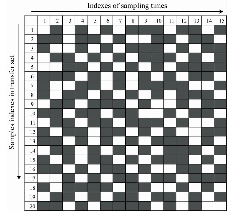
Consider a matrix A_t for m samples with each row as a sample. Two parameters including ratios of the selected sample to the whole sample (r) and the number of selecting times (N) must be focused on. The samples must be randomly selected from A_t to generate the subset. After N times of repeatedly sampling, N subsets of the transfer set can be obtained. This procedure is illustrated in Fig.1 where m=20, r=0.6 and N=15.

Figure 1 shows that the first subset including the 12 samples can be selected among the 20 samples (20×0.6). Further, other 12 samples can be chosen from another sampling index. Thus, after 15 samplings, 15 subsets of the transfer set can be generated. In Fig.1, the probability of each sample is 0.6, which is identical to the value of r. Furthermore, during the sampling, the selected ratio of a sample is r. Thus, after N samplings, the theoretical number of (N_t) of the sample to be selected can be computed as follows

Nt=Nr(1)

The insignificant N_t of cannot extract the sample information in a transfer set, while the substantial value of N_t can increase the computation burden. Thus, an optimal N_t value must be fixed. In this study, N_t is set to 100, which implies the theoretical sampling time of each sample is 100. Thus, the former two parameters can be reduced into a single parameter r. With the value of r, the value of N can be computed as follows

N=100/r(2)

Calibration transfer can be generated for each randomly generated sub-dataset to estimate RMSEV (RMSEV₁). E.g. in Fig.1, 15 RMSEV₁ values can be obtained after 15 sampling times.

After randomly sampling, each sample subset of the transfer set can be applied to the calibration transfer. Thus, the corresponding RMSEV₁ values can be obtained after several sampling times. The subsets with RMSEV₁ values including the corresponding sample can be obtained for one sample. After that, the average RMSEV₁ (mRMSEV₁) can be fixed as the subsets with the sample. For example, in Figure. 1, after 15 samplings, the 2^nd, 4^th , 6^th, 8^th, 9^th, 10^th, 12^th, 13^th and 15^th subsets contain the first sample, and thus mRMSEV₁ of these samples can be obtained to evaluate the transfer power of the first sample. Similarly, mRMSEV₁ of the 1^st, 2^nd, 4^th, 5^th,7^th, 10^th,11^th, 13^th and 14^th subsets can be set as the transfer power of the second sample. Based on this, mRMSEV₁ of each sample can be obtained.

Evidently, after sampling, the samples with low mRMSEV₁ values can be considered candidates for reducing calibration transfer errors. Thus, the samples can be sorted according to their mRMSEV₁ values ascending order, and the samples with low mRMSEV₁ values can be chosen for calibration transfer. The detailed procedure of the proposed method is given as follows:

In Fig.2, the proposed method includes the following four steps: (1) randomly sampling, (2) obtaining RMSEV₁ of each subset, (3) obtaining mRMSEV₁ of each sample, and (4) selecting the samples with low mRMSEV₁ values. In the proposed method, r and the number of samples in the original transfer set (m) must be adjusted in advance.

The spectra of the corn dataset scanned on three NIR spectrometers are downloaded from http://www.eigenvector.com/data/Corn/index.html. Each of the three NIR spectra batches includes 80 samples ranging from 1100 nm to 2498 nm. In the three datasets, mp6 and m5 are assigned as primary and secondary spectra, respectively. Meanwhile, the moisture values are set as y.

For primary spectra with 80 samples, after sorting the values of y, the first sample in each of the four contiguous samples (20 samples) is set aside. Thus, the remaining 60 primary spectra samples are considered the calibration set of primary spectra. Moreover, among 60 samples of calibration set of primary spectra, certain samples are chosen as the transfer sets of primary spectra using the KS method. After generating the transfer set of primary spectra, the samples of the calibration set in secondary spectra with similar y values are assigned as the transfer set of secondary spectra.

Moreover, for 20 samples of primary spectra set aside, the samples of secondary spectra with similar y values as that of the former can be retained. Among 20 samples of secondary spectra, the first and second ones of each two contiguous samples are set as prediction and validation sets, respectively.

For the corn dataset, the number of latent variables is optimized as nine. Additionally, the parameters of m and r must be investigated. Because the sampling subset cannot execute CCA-ICE under the condition of m×r<l, the corresponding RMSEV cannot be generated. Thus, the combinations with m×r≥l must be adopted under different parameter combinations. The results are illustrated below:

Figure 3, shows that at different combinations of m and r, the RMSEV₂ values of the proposed method are nearly lower than those obtained by the KS method. This indicates that the transfer set generated by the KS method can be further refined by using the proposed ER method. In each plot of (c), (d), (e), (f), (g), (h) and (i), with ascending m, RMSEV₂ displays a decreasing trend at m<30. This is because many samples obtained by the KS method facilitate the refinement of ER. Furthermore, after the value of m exceeds 30, RMSEV₂ remains nearly constant. Since selecting many transfer samples may generate redundant information for the calibration transfer, m is set to 30.

In addition to m, r must be investigated. RMSEV₂ at different r values are listed in Fig.4.

In Fig.4, RMSEV₂ achieves the minimal at r=0.6. Thus, r is set to 0.6. After fixing m and r, the variation in RMSEV₂ during different w can be examined. The results are displayed below.

Fig.5 indicates that with the increase in w, RMSEV₂ decreases at first and achieves the minimum at w=28. At last, RMSEV₂ was obtained to be 0.094 2, which is the same as the results without further refinement. Thus, the subset with 28 samples and minimal RMSEV₂ can be set as the optimal subset. Fixing the parameters using the validation set, RMSEP of the prediction set must be applied to examine the effect of ER. The results are displayed as follows:

In Table 1, it is evident that the ER method can refine the transfer set of CCA-ICE with low RMSEV₂ and achieve low RMSEP compared to the KS method. Meanwhile, the commonly used methods such as DS, PDS and SST can also be applied in the ER method. The results are listed in Table 1. In Table 1, DS, PDS and SST utilize ER to refine the transfer set with lower RMSEV₂ and RMSEP than the KS method.

Moreover, to further analyze the power of ER, the random sampling method can be used for testing. In each calibration transfer method including CCA-ICE, DS, PDS and SST, the randomly sampling method is used 100 times. In each loop, the calibration, validation and prediction sets are randomly fragmented into the sizes of 60, 10 and 10, respectively. Then, the original transfer sets are generated from the calibration set through the KS method. Subsequently, the samples in the transfer set are further refined by the ER method, and RMSEV₂ of the validation set is used to determine the number of samples to be retained. Finally, the refined and non-refined samples are applied to transfer the prediction set. After 100 randomly samplings, RMSEP of KS and ER at different m can be computed as follows:

In Fig.6, it is evident that for each transfer method, including CCA-ICE, DS, PDS and SST, at different numbers of m, the RMSEP values of ER are lower than those of KS. Among the four calibration transfer methods, CCA-ICE can generate low prediction errors. CCA-ICE transfers the informative components extracted by the partial least squares (PLS) model. Moreover, the backward refinement can further reduce the errors in a prediction set. For DS and SST, with increasing m, RMSEP values of KS display a decreasing trend, while ER’s values remains nearly constant. This implies that ER can select key samples for calibration transfer through DS and SST with low errors. In Fig.6(c), although the errors of PDS obtained by KS are larger than those of CCA-ICE, DS and SST, ER can reduce prediction errors by refining the samples.

A new transfer set refinement method ER was proposed based on MPA. Initially, ER generated several subsets for the calibration transfer. Subsequently, the average errors of subsets containing this sample were obtained for each sample.

Finally, samples with low average errors were selected as the refined transfer set. The corn dataset was used to test the proposed method. The results indicated that the calibration transfer methods, including CCA-ICE, DS, PDS and SST could reduce prediction errors. Hence, ER can effectively refine the transfer set in calibration transfer.

References

[1] A Boldrin, T Fitamo, J M Triolo et al. Water Research, 119, 242(2017).
[2] S Liu, S Wang, Y Yuan et al. Infrared Physics and Technology, 106, 103(2020).
[3] J Shi, S Wu, F Zhang et al. Food Chemistry, 274, 925(2019).
[4] Y Chen, X D Sun, H L Wu et al. Chemometrics and Intelligent Laboratory Systems, 194, 103(2019).
[5] L M S L Oliveira, J T C Rocha, R R T Rodrigues et al. Chemometrics and Intelligent Laboratory Systems, 166, 7(2017).
[6] E Garbin, G Marchesini, L Serva et al. Italian Journal of Animal Science, 17, 66(2017).
[7] Yu-ting CAO, Chen LIANG, Zhong ZHAO et al. Spectroscopy and Spectral Analysis, 37, 1587(2017).
[8] K D T M Milanez, D S Nascimento, T C A Nobrega et al. Microchemical Journal, 133, 669(2017).
[9] X Lou, H Yang, J Yang et al. Analytical Letters, 52, 2188(2019).
[10] J Bin, W Fan, X Li et al. Analyst, 142, 2229(2017).
[11] Z Chen, W Du, L Zhong et al. Analytica Chimica Acta, 690, 64(2011).
[12] Yi-yun CHEN, Tian-ci QI, Rui-Ying ZHAO et al. Spectroscopy and Spectral Analysis, 37, 2133(2017).
[13] B Deng, H Long, T Tang et al. International Journal of Molecular Sciences, 20, 955(2019).
[14] B Deng, H Lu, C Tan et al. Chemometrics and Intelligent Laboratory Systems, 172, 223(2018).
[15] W Chen, F Zhang, R Zhang et al. Chemometrics and Intelligent Laboratory Systems, 171, 234(2017).
Set citation alerts for the article
Please enter your email address
© Copyright 2018-2021 | Chinese Laser Press. All Rights Reserved 沪ICP备15018463号-20