Researchers and photographers have long sought to unravel transient events on an ultrashort time scale using ultrafast imaging. From the early observations of a galloping horse¹ to capturing the electronic motions in nonequilibrium materials,² this research area has continuously developed for over 140 years. Currently, with the aid of subfemtosecond (fs, 10−15s) lasers^3,4 and highly coherent electron sources,^5,6 it is possible to simultaneously achieve attosecond (as, 10−18s) temporal resolution and subnanometer (nm, 10−9m) spatial resolution.^7,8 Ultrafast imaging holds great promise for advancing science and technology, and it has already been widely used in both scientific research and industrial applications.

Ultrafast imaging approaches can be classified into stroboscopic and single-shot categories. For transient events that are highly repeatable, reliable pump-probe schemes are used to explore the underlying mechanisms. Unfortunately, this strategy becomes ineffective in circumstances with unstable and even irreversible dynamics, such as optical rogue waves,⁹ irreversible structural dynamics in chemical reactions,^10,11 and shock waves in inertial confinement fusion.¹² To overcome this technical limitation, a variety of single-shot ultrafast imaging techniques with the ability to visualize the evolution of two-dimensional (2-D) spatial information have been proposed.¹³ Based on their methods of image formation, these imaging techniques can be further divided into two categories. One is the direct imaging without the aid of computational processing, such as ultrafast framing/sampling cameras,¹⁴ femtosecond time-resolved optical polarimetry,¹⁵ and sequentially timed all-optical mapping photography (STAMP).¹⁶ The other category is reconstruction imaging, in which dynamic scenes are extracted or recovered from the detected results by specific computational imaging algorithms, including holography,¹⁷ tomography,¹⁸ and compressed sensing (CS)-based photography.^19,20 As summarized in Ref. 13, although direct imaging methods are still important and reliable for capturing transient events in real time, an increasing number of reconstruction imaging approaches have achieved substantial progress in various specifications, such as imaging speed, number of pixels per frame, and sequence depth (i.e., frames per shot).

Among the various reconstruction imaging modalities, compressed ultrafast photography (CUP) advantageously combines the super-high compression ratio of sparse data achieved by applying CS and the ultrashort temporal resolution of streak camera techniques. CUP has achieved a world record imaging speed of 10 trillion frames per second (Tfps), as well as a sequence depth of hundreds of frames simultaneously with only one shot.¹⁹ Moreover, a series of ultrafast diffractive and microscopic imaging schemes with electron and x-ray sources have been proposed to extend the modality from optics to other domains. In recent years, CUP has emerged as a promising candidate for driving next-generation single-shot ultrafast imaging.

Covering recent research outcomes in CUP and its related applications since its first appearance in 2014,¹⁹ this review introduces and discusses state-of-the-art imaging techniques, including their principles and applications. The subsequent sections are arranged as follows. In Sec. 2, we describe the working principle of CUP and discuss mathematical models of the data acquisition and the image reconstruction processes. In Secs. 3 and 4, we review technical improvements and extensions of this technique so far, respectively. The technical improvements are explained with regard to the data acquisition and the image reconstruction, whereas the technical extensions of CUP combine a variety of techniques. In Sec. 5, related applications of CUP are described and discussed, not only for optical measurements but also for information security protection. Finally, we conclude this review in Sec. 6 and speculate on future research directions.

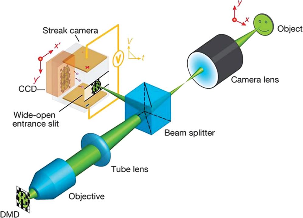
A CUP experiment can be completed in two steps: data acquisition and image reconstruction. A simple experimental diagram for data acquisition is shown in Fig. 1.¹⁹ A dynamic scene is first imaged on a digital micromirror device (DMD) by a camera lens and a 4f imaging system consisting of a tube lens and a microscope objective, and then it is encoded in the spatial domain by the DMD. Subsequently, the encoded dynamic scene reflected from the DMD is collected by the same 4f imaging system. Finally, it is deflected and measured by a streak camera.

A DMD consists of hundreds of thousands of micromirrors; each of which can be individually rotated with ±12deg that represents an on or off state.²¹ When a pseudorandom binary code is loaded onto a DMD, these micromirrors can be turned on or off accordingly, thus a dynamic scene projected on the DMD can be spatially encoded. In CUP acquisition, the entrance slit of the streak camera is fully opened (∼5mm), and a scanning control module in the streak camera provides a sweeping voltage that linearly deflects the photoelectrons induced by the dynamic scene according to their arrival times. The temporally sheared image operated by the streak camera is captured by a CCD in a single exposure. In the CUP experiment, the pseudorandom binary code generated by the DMD is fixed. Consequently, data acquisition is divided into three steps, which can be described by a forward model. As shown in Fig. 2(a), this procedure can be mathematically described as follows: the three-dimensional (3-D) dynamic scene I(x,y,t) is first imaged onto an intermediate plane, on which the intensity distribution of the intermediate image is identical to that of the original scene under the assumption of ideal optical imaging with unit magnification. The intermediate image is successively processed by a mask containing pseudorandomly distributed, squared, and binary-valued elements at the intermediate image plane. The image intensity distribution after this operation is formulated as Here, Ci,j is an element of the matrix representing the coded mask, i, j are the matrix element indices, and d is the mask pixel size that is equivalent to a binned DMD or CCD pixel. For both dimensions, the rectangular function (rect) is defined as Then, the encoded dynamic scene is sheared by the streak camera in the time domain by applying a voltage ramp along the vertical y′ axis and can be expressed as where v is the shearing velocity of the streak camera. Finally, the scene is spatially and temporally integrated over each camera pixel and the exposure time, respectively, and forms a 2-D image on the detector. Thus, the optical energy E(x′,y′) of the integrated 2-D image is Accordingly, voxelization of I(x,y,t) into Ii,j,τ can be expressed as where Δt=d/v. Given the prerequisite of perfect registration of the mask elements and the camera pixels, a voxelized expression of E(x′,y′) can be yielded by combining Eqs. (1)–(4) as follows: where Cx′,y′−τIx′,y′−τ,τ indicates a coded, sheared scene. In general, a spatial encoding operator C, a temporal shearing operator S, and a spatiotemporal integration operator T are introduced and form a 2-D image E(x′,y′), which is expressed as Here, for simplicity, a notation is introduced O=TSC.

It is noteworthy that, given a coded mask with dimensions of Nx×Ny, the input scene I(x,y,t) can be voxelized into a matrix form with dimensions Nx×Ny×Nt under the assumption of ideal optical imaging with unit magnification, where Nx, Ny, and Nt are the numbers of voxels along x, y, and t, respectively. Therefore, the measured E(x′,y′) has dimensions Nx×(Ny+Nt−1), and the spatial resolution of CUP is mainly determined by Nx and Ny or the mask pixel size, d, while the temporal resolution is restricted by Nt, which is related to the shearing velocity of streak camera, v.

Given the prior knowledge of the forward model, the image reconstruction tries to estimate the unknown dynamic scene I(x,y,t) from the captured 2-D image E(x′,y′) by solving the linear inverse problem of Eq. (6). The number of elements in the 3-D dynamic scene I(x,y,t) is approximately two orders of magnitude larger than that in the 2-D image E(x′,y′).¹⁹ Therefore, the inverse problem of Eq. (6) is underdetermined, which suffers from great uncertainty to reconstruct the real result of I(x,y,t) from E(x′,y′) by a traditional approach based on the parameters T, S, and C. CUP introduces CS theory to solve this problem.^22,23 Here, CS makes full use of the sparsity of I(x,y,t) in a certain domain to recover the original scene. Sparsity in a certain domain means that most elements are zeros, whereas only a few elements are nonzeros. Consider the case where I(x,y,t) has n elements in the original domain and s nonzero elements in the sparse domain, whereas E(x′,y′) has m elements, where n≫s and n>m>s. The fact that m is larger than s makes it possible to solve the inverse problem of Eq. (6). To practically solve this problem, CUP finds the best I(x,y,t) using a CS algorithm in a certain sparse domain under the condition of Eq. (6), which is shown as where Φ[I(x,y,t)] is the expression of I(x,y,t) in a sparse domain. Usually, the domain can be in various forms to achieve a sparsity as high as possible, including the space, the time, or both. Based on the theory of stable signal recovery from incomplete and inaccurate measurements,^23–25 the original I(x,y,t) can be completely recovered when where f is a constant that is correlated with the number of elements n, and μ is the mutual coherence between the sparse basis of I(x,y,t) and the measurement matrix that is dependent on the operators C, S, and T. To recover I(x,y,t), CUP first sets its initial guess as a point in an n-dimensional space, denoted as I0. Starting from the initial point I0, the CS algorithm can search for the destination point IL, and this optimization process can be described as follows: the intermediate point Ii is updated in each iteration until Ii reaches the proximity of IL, as shown in Fig. 2(b). In addition, the search paths should obey Eq. (7), but they will be different in different CS algorithms. For these search paths, there exist at least five major classes of computational techniques: greedy pursuit, convex relaxation, Bayesian framework, nonconvex optimization, and brute force. The details can be found in Ref. 26. For different CS algorithms, the final IL points are different, which indicates that an optimal CS algorithm exists. The difference between IL and the original I can be utilized as the standard for judging the algorithm’s quality. Last but not least, noise always exists in experimental data. Moreover, Eq. (8) is often unsatisfied due to the large compression ratio caused by transforming the 3-D data cube I(x,y,t) into the 2-D data E(x′,y′), as shown in Fig. 2(a). Therefore, Eq. (7) can be further written as where ‖.‖2 denotes the l2 norm and δ is the value of the error.

Based on the data acquisition and image reconstruction procedures with a single-shot operation, the CUP system with the configuration shown in Fig. 1 can achieve an imaging speed as high as 100 billion fps and a sequence depth of 350. For each frame, the spatial resolution is ∼0.4 line pairs per mm in a 50-mm×50-mm field of view (FOV). CUP has itself empowered outstanding performance as a single-shot ultrafast imaging technique, but many technical improvements have emerged.

In this section, we review recent technical improvements in the CUP technique from two aspects of CUP’s experimental operation. In Sec. 3.1, we discuss a few strategies for data acquisition inspired by Eq. (8), as well as the fastest CUP system with a streak camera, which has femtosecond temporal resolutions. In Sec. 3.2, we review improvements in image reconstruction algorithms.

Equation (8) holds the key to improving data acquisition. For a given dynamic scene I(x,y,t), the coefficient of nonzero elements in the original domain, f, and the number of nonzero elements in the sparse domain, s, are constants. Fortunately, improvements can be realized by reducing the mutual coherence, μ, or increasing the measured number of elements, m. Based on this principle, a few novel approaches have been proposed.

The parameter μ represents the mutual coherence between the sparse basis of I(x,y,t) and the measurement matrix. The measurement matrix mainly depends on the encoding operator C (i.e., the random codes on the DMD), which indicates that CUP performance can be improved by optimizing the random codes. Yang et al. adopted a genetic algorithm (GA) to optimize the codes.²⁷ The GA is designed to self-adaptively find the optimal codes in the search space and eventually obtain the global solution. Utilizing the optimized codes, CUP needs three steps to recover a dynamic scene, as shown in Fig. 3(a). First, a dynamic scene is set as the optimization target. This scene can be different from the real dynamic scene but must maintain the same sparse basis. This optimization target scene consists of the images reconstructed by CUP using the random codes. Second, the GA is utilized to optimize the codes according to the optimization target, which represents the reconstructed images in step I. These reconstructed images constitute a simulated scene, which is then recovered by computer simulation with many sets of random codes. Each set of random codes is regarded as an individual, and these individuals constitute a group. Here, the GA simulates biological evolution to find the optimal codes. The details can be found in Ref. 27. Finally, using the optimal codes obtained in step II, CUP records the dynamic scene for a second time.

Figures 3(b) and 3(c) show reconstructed results using the optimal codes and random codes, respectively. Here, the dynamic scene is a time- and space-evolving laser pulse with a pulse width of 3 ns and a central wavelength of 532 nm, and the laser spot is divided into two components in space by a thin wire. The result obtained by the optimal codes has less noise and is more distinct in the spatial profile than that obtained by the random codes. However, a total of three steps have been performed for one optimization, so this method demands that the dynamic scene be repeatable twice. For some nonrepeatable scenes, a similar dynamic scene should be found in advance, and it should have the same sparse basis as the real dynamic scene.^30–32 One point to note is that the decrease in μ realized by optimizing the codes using the GA is somewhat limited, because it can only optimize operator C; it is invalid to other operators that constitute the measurement matrix.

As shown in Eq. (8), the parameter m represents the number of elements in E(x′,y′). For a given dynamic scene, m is a constant if the scene is encoded by a single set of random codes, as is shown in Fig. 2(a). To increase m, more sets of random codes can be utilized to simultaneously encode the dynamic scene: this method is called multiencoding CUP.²⁹ In this method, as shown in Fig. 4, an ultrafast dynamic scene is divided into several replicas, and each replica is encoded by an independent encoding mask. Finally, these replicas are individually imaged after temporal shearing. Thus, Eq. (5) can be further formulated in matrix form as [E1(x′,y′)E2(x′,y′)⋮Ek(x′,y′)]=[TSC1TSC2⋮TSCk]I(x,y,t),(10)where k is the number of encoding masks, Ek(x′,y′) is the k’th measured 2-D image, and Ck, S, and T denote the k’th spatial encoding operator, the temporal shearing operator, and the spatiotemporal integration operator, respectively. In this condition, m is increased k times, whereas the mutual coherence, μ, is decreased to a limited extent by optimizing the codes. Compared with schemes for decreasing μ, increasing m is a more effective method.

Coincidently, the lossless encoding CUP (LLE-CUP) proposed by Liang et al.³³ can also be regarded as a method to increase m. There are three views in LLE-CUP: the dynamic scene in two of the views is encoded by complementary codes and is then sheared and integrated by the streak camera, and the results are called the sheared views. The dynamic scene in the third view is just integrated by an external CCD, and the result is called the unsheared view. Mathematically, only the sheared views have an effect on extracting the 3-D datacube from the compressed 2-D image, whereas the unsheared view is used to restrict the space and intensity of the reconstructed image. In this method, the sheared views provide different codes for each acquisition channel, and each image is reconstructed by its own codes. Nevertheless, the unsheared view still improves the image reconstruction quality in some situations, and it is adopted in a few approaches.^34,35

It is worth mentioning that both schemes can effectively improve CUP’s performance by increasing the sampling rate. Moreover, as demonstrated in Ref. 29, a multiencoding strategy can break through the original temporal resolution limitation of the temporal deflector (e.g., the streak camera), which was formerly considered a restriction on the frame rate of a CUP system. The reconstructed image quality is significantly improved by increasing m, but the spatial resolution may decrease when the CCD is divided into several subareas to image the dynamic scenes in these channels. However, if the channels are arranged sophisticatedly or the FOV can be sacrificed, the spatial resolution can reach a balanced value. Moreover, the synchronization between different channels is very crucial for realizing the achievable temporal resolution.

One of the most important characteristics of a CUP system is its ultrafast imaging speed, which is definitively determined by the temporal deflector. Based on a prototype of CUP, Liang et al. recently established a trillion-frame-per-second compressed ultrafast photography (T-CUP) system and realized real-time, ultrafast, passive imaging of temporal focusing with 100-fs frame intervals in a single camera exposure.³⁴ A diagram of the T-CUP system is shown in Fig. 5. Similar to the first-generation CUP system (Fig. 1), it performs data acquisition and image reconstruction, but an external CCD is installed on the other side of the beam splitter. A 3-D spatiotemporal scene is first imaged by the beam splitter to form two replicas. The first replica is directly recorded by the external CCD by temporally integrating it over the entire exposure time. In addition, the other replica is spatially encoded by a DMD, and then sent to a femtosecond streak camera with the highest temporal resolution of 200 fs, where the entrance slit is fully opened, and the scene is sheared along one spatial axis and recorded by a detector. With the aid of reconstruction algorithms to solve the minimization problem, one can obtain a time-lapse video of the dynamic scene with a frame rate as high as 10 Tfps. In a CUP system, the imaging speed mainly depends on the temporal resolution of the streak camera. Therefore, by varying the temporal shearing velocity of the streak camera, the frame rate can be widely varied from 0.5 to 10 Tfps, with corresponding T-CUP temporal resolutions from 6.34 to 0.58 ps.

Foremost, it is noteworthy that all reconstructed scenes using the T-CUP system are accurate to 100 fs in frame interval, with a sequence depth (i.e., number of frames per exposure) of more than 300. To the best of our knowledge, this is the world’s best combination of imaging speed and sequence depth. On the other hand, it should be noted that a streak camera needs photon-to-electron and electron-to-photon conversion for 2-D imaging, and this limitation confines the pixel count of each reconstructed image to tens of thousands.

Because CS theory is key to CUP, efforts to improve the reconstruction algorithms for performance improvement have been important. One example is optimizing the search path to seek a better CS algorithm, which has resulted in the proposed use of the augmented Lagrangian (AL) algorithm.³⁶ In addition, an alternative scheme is confining the search path within a certain scope, which is called the space- and intensity-constrained (SIC) reconstruction method.³⁷

Heretofore, all CS algorithms for CUP were based on total variation (TV) minimization, which is a convex relaxation technique. TV minimization can make the recovered image quality sharp by preserving boundaries more accurately,^38,39 which is essential to characterize the reconstructed images. The original tool for image reconstruction in CUP was a two-step iterative shrinkage/thresholding (TwIST) algorithm.²⁸ The TwIST algorithm is a quadratic penalty function method and can transform Eq. (9) into minI{Φ[I(x,y,t)]TV+β2‖E(x′,y′)−OI(x,y,t)‖22},(11)where Φ[I(x,y,t)]TV is the TV regularizer and β is the penalty parameter, with β>0. Alternatively, Eq. (9) can also be written in Lagrangian function form and given as minI{Φ[I(x,y,t)]TV−λ[E(x′,y′)−OI(x,y,t)]},(12)where λ is the Lagrange multiplier vector and E(x′,y′)−OI(x,y,t) is written as a vector. When calculating the derivatives of I(x,y,t) in Eqs. (11) and (12), this relationship can be expressed as E(x′,y′)−OI(x,y,t)=−1βλ.(13)Here, the value of E(x′,y′)−OI(x,y,t) is used to illustrate the feasibility of the image reconstruction, and a smaller value corresponds to greater feasibility. It is easy to see from Eq. (13) that increasing β can improve the feasibility but will cause ill conditions for the quadratic penalty function.⁴⁰ To avoid this problem, an AL function method has been proposed,³⁹ presented as minI{Φ[I(x,y,t)]−γ[E(x′,y′)−OI(x,y,t)]+β2‖E(x′,y′)−OI(x,y,t)‖22},(14)where γ is a variable Lagrange multiplier vector. By following the transformation from Eqs. (11)–(13), it is easy to obtain E(x′,y′)−OI(x,y,t)=−1β(λ−γ).(15)Compared with Eq. (13), the value of E(x′,y′)−OI(x,y,t) in Eq. (15) depends on both β and γ. By optimizing γ through iteration, it is easy to find the minimum. Therefore, compared to the TwIST algorithm, the AL algorithm can provide higher image reconstruction quality.

To further validate the improvement in the image reconstruction quality, a superluminal propagation of noninformation was recorded in Ref. 36. As shown in Fig. 6(a), a femtosecond laser pulse obliquely illuminates a transverse stripe pattern at an angle of ∼38deg with respect to the surface normal, and a CUP camera is vertically positioned for recording. Figures 6(b) and 6(c) show the experimental results reconstructed by the AL algorithm and the TwIST algorithm, respectively. Clearly, the images reconstructed by the TwIST algorithm have more artifacts, whereas those reconstructed by the AL algorithm are more faithful to the true situation. The AL algorithm opens up new approaches to solving this inverse problem, such as gradient projection for sparse reconstruction.⁴¹ In the near future, more studies will surely be carried out to further optimize image reconstruction algorithms.

A scheme proposed by Zhu et al. confines the search path within certain scopes and is accordingly named the SIC reconstruction algorithm.³⁷ This method operates in a spatial zone M, and the values of pixels outside of this region are set as zeros. The spatial zone M is extracted from the unsheared spatiotemporally integrated image of the dynamic scene, recorded by an external CCD, which is similar to the hardware configuration in Sec. 3.1.3. In addition, the values of pixels less than the intensity threshold s, even in zone M, are set to zero. By using the penalty function framework, the SIC reconstruction algorithm can be written as minI∈M,I>s{Φ[I(x,y,t)]TV+β2‖E(x,y)−OI(x,y,t)‖22}.(16)Here, zone M is chosen by an adaptive local thresholding algorithm and a median filter. The threshold is chosen from a couple of candidates between 0 and 0.01 times of the maximal pixel value. The criterion for these values is the minimal root-mean-square error between the reconstructed integrated images obtained by the algorithm and the unsheared integrated image obtained by the external CCD.

To demonstrate the advantages of the SIC reconstruction method, a picosecond laser pulse propagation was captured by a derivative of the primary CUP system, and the reconstructed results by the unconstrained (i.e., TwIST) and constrained (i.e., SIC) algorithms are shown in Figs. 7(a) and 7(b), respectively. Clearly, the SIC reconstructed image maintains sharper boundaries than the TwIST reconstructed image. Moreover, the normalized intensity profiles in Fig. 7(c) further show that the spatial and temporal resolutions are simultaneously improved using the SIC algorithm.

In mathematical models of CUP, CS offers a scheme that allows the underdetermined reconstruction of sparse scenes.⁴² Since CUP uses a linear and undersampled imaging system, such a model can be flexibly extended to other systems to address their limitations. Three representative works in recent years are presented here to inspire researchers. The first extension, described in Sec. 4.1, originates from the combination of CUP and STAMP to realize ultrafast spectral–temporal photography based on CS. Next, similar to its usage in the CUP system, CS is introduced into microscopic systems based on electron sources to explore ultrafast structural dynamics in a single shot, as reviewed in Sec. 4.2. Finally, a novel all-optical ultrahigh-speed imaging strategy that does not employ a streak camera is described and discussed in Sec. 4.3.

As introduced in Sec. 1, both direct and computational imaging techniques have achieved remarkable progress in recent years, but they have seemed to develop independently and without intersection. In the early 2019, Lu et al. creatively proposed a new compressed ultrafast spectral–temporal (CUST) photography system⁴³ by merging the modalities of CUP and STAMP. Combining the advantages of these two ultrafast imaging systems, the CUST system, shown schematically in Fig. 8, provides both an ultrahigh frame rate of 3.85 Tfps and a large number of frames. The CUST system consists of three modules: a spectral-shaping module (SSM), a pulse-stretching module (PSM), and a so-called “compressed camera.” In the SSM, a femtosecond laser pulse passes through a pair of gratings and a pulse shaping system with a 4f configuration. On the Fourier plane of the 4f system, a slit is positioned to select a designated spectrum of the femtosecond pulse. In the PSM, the femtosecond pulse is stretched by another pair of gratings to generate a stretched picosecond-chirped pulse as illumination. The “compressed camera” is similar to that in the CUP system, but the main difference is that the streak camera is replaced by a grating to disperse the spatially encoded event at different wavelengths. Because the illumination pulse is chirped linearly, it ensures a one-to-one linear relationship between the temporal and wavelength information. Finally, a CS algorithm is employed to reconstruct the dynamic scene, much as in CUP. By recording ultrafast spectrally resolved images of an object, the CUST system can acquire 60 spectral images with a 0.25-nm spectral resolution on approximately a picosecond timescale.

The temporal solution of the CUST technique mainly depends on the chirp ability of the pulse-shaping system and the spectral resolution of the compressed camera; therefore, the imaging speed can be flexibly adjusted by tuning the grating components. In comparison to STAMP, CUST offers more frames. However, since the CUST system uses a chirped pulse as illumination, it cannot measure a self-emitting event, such as fluorescence, or the color of the object.

Understanding the origins of many ultrafast microscopic phenomena requires probing technologies that provide both high spatial and temporal resolution simultaneously. Based on the inherent limitations of the elementary particles in the imaging processes, photons and electrons have accounted for the most powerful imaging tools, but the two are dissimilar in terms of the spatial and temporal domains they can access. Photons can be used for extremely high (up to attosecond) temporal studies, whereas accelerated electrons excel in forming images with the highest spatial resolution (sub-angstrom) achieved so far. In recent decades, many researchers have focused on merging conventional electron diffraction and microscopy systems with ultrafast lasers, and a variety of structurally related dynamics have been explored. Unfortunately, these systems still suffer from the limitations of multiple-shot measurements and synchronization-induced timing jitter.

To overcome the limitations in this research field, solutions have been proposed based on the methodology of CUP. Qi et al. proposed a new theoretical design, named compressed ultrafast electron diffraction imaging (CUEDI),⁴⁴ which, for the first time, subtly combines an ultrafast electron diffraction (UED) system with the CUP modality. As shown in Fig. 9(a), by utilizing a long-pulsed laser to generate the probe electron source and inserting an electron encoder between the sample and the streak electric field, CUEDI completes the measurement in a single-shot, which eliminates the relative time jitter between the pump and probe beams. In addition, Liu et al. in 2019 added CS to a laser-assisted transmission electron microscopy (TEM) setup to create two related novel schemes, named single-shearing compressed ultrafast TEM (CUTEM) and dual-shearing CUTEM (DS-CUTEM),⁴⁵ which are shown in Figs. 9(b) and 9(c), respectively. In each scheme, the projected transient scene experiences encoding and shearing before reaching the detector array. However, an additional pair of shearing electrodes is inserted before the encoding mask in the DS-CUTEM scheme, which is used to shear the dynamic scene in advance, and thus a more incoherent measurement matrix is generated by the encoding mask. Therefore, the mutual coherence of the scene in DS-CUTEM is even smaller than that in CUTEM. Based on these analytical models and simulated results, single-shot ultrafast electronic microscopy with subnanosecond temporal resolution could be realized by integrating CS-aided ultrafast imaging modalities with laser-assisted TEM.

Because a streak camera is used in previous CUP systems, photon–electron–photon conversion cannot be avoided, thus deteriorating the reconstructed image quality in each frame. To overcome this limitation, Liu et al. in 2019 developed single-shot compressed optical-streaking ultrahigh-speed photography (COSUP),⁴⁶ which is a passive-detection computational imaging modality with a 2-D imaging speed of 1.5 million fps (Mfps), a sequence depth of 500, and a pixel count of 1000×500 per frame. In the COSUP system, the temporal shearing device is a galvanometer scanner (GS), not a streak camera. As shown in Fig. 10, the GS is placed at the Fourier plane of the 4f system, and, according to the arrival time, it temporally shears the spatially encoded frames linearly to different spatial locations along the x-axis of the camera. Moreover, COSUP and CUP share the same mathematical model.

Compared with CUP, the temporal resolution of the COSUP system is much lower since it is currently limited by the linear rotation voltage of the GS. However, because COSUP avoids the electronic process in a streak camera, its spatial resolution is over 20 times higher. Importantly, the ingenious design of optical streaking provides a new approach for improving the spatial resolution of CUP-like systems, for example, with optical Kerr effect gates and Pockels effect gates. Moreover, because of the simplification of components in COSUP, it provides a cost-effective alternative way to perform ultrahigh-speed imaging. For the future, a slower COSUP system combined with a microscope holds great potential to enable such bioimaging feats as high-sensitivity optical neuroimaging of action potential propagation and using nanoparticles for wide-field temperature sensing in tissue.^47–49

As explained in the previous sections, by synergizing CS and streak imaging, the CUP technique can realize single-shot ultrafast optical imaging in receive-only mode. In recent years, manifold improvements in this technique have enabled the direct measurement of many complex phenomena and processes that were formerly inaccessible to ultrafast optics. Several representative areas of investigation are reviewed in this section, including capturing the flight of photons, imaging at high speed in 3-D, recording the spatiotemporal evolution of ultrashort pulses, and enhancing image information security.

The capture of light during its propagation is a touchstone for ultrafast optical imaging techniques, and a variety of schemes have been proposed to accomplish it, including CUP. Using the first-generation CUP system described in Sec. 2, Gao et al. demonstrated the basic principles of light propagation by imaging laser pulses reflecting, refracting, and racing in different media in real time for the first time. Further, they modified the setup with a dichroic filter design to develop the spectrally resolvable CUP shown in Fig. 11(a) and successfully recorded the pulsed-laser-pumped fluorescence emission process of rhodamine.¹⁹ These results are shown in Fig. 11(b). With the creation of LLE-CUP, described in detail in Sec. 3.1.2, Liang et al. recorded a photonic Mach cone propagating in scattering material for the first time,³³ presenting the formation and propagation images shown in Fig. 11(c). The experimental results are in excellent agreement with theoretical predictions by time-resolved Monte Carlo simulation.^50–52 In addition, although the propagation of photonic Mach cones had been previously observed via pump-probe methods,^53,54 this was the first time that a single-shot, real-time observation of traveling photonic Mach cones induced by scattering was achieved. By capturing light propagation in scattering media in real-time, CUP demonstrated great promise for advancing biomedical instrumentation for imaging scattering dynamics.^55–57

3-D imaging is used in many applications,^58–67 and numerous techniques have been developed, including structured illumination,^68,69 holography,⁷⁰ streak imaging,^71,72 integral imaging,⁷³ multiple camera or multiple single-pixel detector photogrammetry,^74,75 and time-of-flight (ToF) detection based on kinect sensors⁷⁶ and single-photon avalanche diodes.^77,78 Recently, these 3-D imaging techniques have been increasingly challenged to capture information fast.

ToF detection is a common method of 3-D imaging that is based on collecting scattered photons from multiple shots of objects carrying a variety of tags. Although it offers high detection sensitivity, multiple-shot acquisition still falls short in imaging fast-moving 3-D objects. To overcome this difficulty, single-shot ToF detection approaches have been developed.^79–84 However, within the limited imaging speeds of CMOS cameras and the illuminating pulse widths, 3-D imaging speeds have been limited to ∼30Hz, with a depth resolution of ∼10cm. Liang et al. developed a new 3-D imaging system, named ToF-CUP,³⁵ that satisfied the single-shot requirement in ToF detection using a CUP device. In the ToF-CUP system, the CUP camera detects the photons backscattered from a 3-D object illuminated by a laser pulse. By calculating the times of the round-trip ToF signals between the illuminated surface and detector, the relative depths of the light incidence points on the object’s surface can be recovered. The experimental results for two static models and a dynamic two-ball rotation are shown in Fig. 12. Especially in dynamic detection, the ToF-CUP system captured the rotation of this two-ball system by sequentially acquiring images at a speed of 75 volumes per second. Each image was reconstructed to a 3-D (x,y,z) datacube, and these datacubes were further formed into a time-lapse four-dimensional (x,y,z,t) datacube.

The ToF-CUP system is an ingenious variation of the CUP system and exhibits markedly superior performance in imaging speed (75 Hz) and depth resolution (10 mm) for single-shot 3-D imaging. It is believed that the superiority of CUP can effectively advance existing 3-D imaging technologies beyond present bottlenecks. Based on ToF-CUP, more 3-D CUP systems will be proposed in the future, such as combining a CUP camera with a structured illumination system or a holographic system. Given the ability of ToF-CUP in 3-D imaging, it is promising to be widely used in bioimaging, remote sensing, machine vision, and so on.

The spatiotemporal measurement of ultrashort laser pulses provides important reference values for studies in ultrafast physics, such as explorations of second harmonic generation. In studying such physical processes, the characteristics of an ultrashort laser pulse are quite important, including its frequency information, temporal information, spatial information, and their interrelationship. However, most technologies for laser pulse measurement provide only temporal intensity information without spatial resolution, including optical autocorrelators, devices using spectral phase interferometry for direct electric-field reconstruction,⁸⁵ and frequency-resolved optical gating devices.⁸⁶ Since these mainstream techniques are generally limited by direct integration over the transverse coordinates, they can obtain only the temporal information of ultrashort laser pulses.

To extend the information that can be achieved from one image, the CUP technique was employed to simultaneously explore the spatiotemporal information of laser pulses with multiple wavelength components.⁸⁷ A Ti:sapphire regenerative amplifier and a barium borate crystal were used to generate picosecond laser pulses with a fundamental central wavelength of 800 nm and second harmonics of 400 nm. Consequently, the spatiotemporal intensity evolution of the generated dual-color picosecond laser field was obtained as shown in Fig. 13(a). Clearly, CUP precisely obtained not only the pulse durations and spatial evolution of subpulses but also the time delay between them.

In a related effort, Liang et al. utilized the T-CUP system introduced in Sec. 3.1.3 to realize real-time, ultrafast, passive imaging of temporal focusing.³⁴ There are two major features in temporal focusing: the shortest pulse width locates at the focal plane of the lens⁸⁸ and the angular dispersion of the grating induces a pulse front tilt.⁸⁹ To observe the phenomenon experimentally, a typical temporal focusing scenario of a femtosecond laser pulse was generated with a diffractive grating and a 4f imaging system. Actually, the pulse front tilt in this experiment was determined by the overall magnification ratio of the 4f system, the central wavelength of the ultrashort pulse, and the grating period.^90,91 From the front-view and side-view detections, the T-CUP system respectively recorded the impingement of the tilted laser pulse front sweeping along the y-axis of the temporal focusing plane and the full evolution of the pulse propagation across this focusing plane, as shown in Fig. 13(b).

Compared with other single-shot ultrafast imaging techniques,^{16–18,92–96} it is obvious that T-CUP is currently the only technology capable of observing temporal focusing in real time. Unlike STRIPED FISH,⁹⁷ CUP avoids the need for a reference laser pulse, which provides a simpler measurement system. Moreover, based on the spectral response of the streak camera, CUP can measure laser fields with multiple wavelengths covering a wide spectral range. Thus, CUP clearly reveals the complex evolutions of ultrafast dynamics, paving the way for single-shot characterization of ultrashort laser fields in different circumstances.

Information and communication security are critical for national security, enterprise operations, and personal privacy, but the advent of supercomputers and future quantum computers has made it much easier to attack digital information in repositories and in transmission. Recently, a quantum key distribution (QKD) cryptographic technique was developed to protect information and communication security,⁹⁸ and a series of studies have demonstrated that this cryptographic technique can maintain security in a variety of research fields.^99–103 In contrast to traditional public-key cryptography methods, such as elliptic curve cryptography, the digital signature algorithm, and the advanced encryption standard, a QKD system uses quantum mechanics to guarantee secure communication by enabling two parties to produce a shared random secret key known only to them.^98,104,105 However, the relatively low-key generation rate of QKD greatly limits the information transmission bandwidth.¹⁰⁶

To improve this limitation, Yang et al. developed a new hybrid classical-quantum cryptographic scheme by combining QKD and a CS algorithm that improves the information transmission bandwidth.¹⁰⁷ This approach employs the mathematical model of CUP in Fig. 2, where the quantum keys generated by QKD were used to encrypt and decrypt compressed 3-D image information, and a CS theory was utilized to encode and decode ciphertext. As shown in Fig. 14, the quantum key generated by the QKD system is transmitted by the quantum channel, whereas the ciphertext encoded by the CS algorithm is transmitted by the classical channel. Because a CS algorithm is a nondeterministic polynomial hard (NP-hard) problem and this approach is looking for an approximate solution, the CS-QKD system can obtain higher encryption efficiency under low key generation rate conditions. Based on analyses of the normalized correlation coefficient in several attack trials, the CS-QKD scheme has been proven to effectively improve the information transmission bandwidth by a factor of approximately three and to ensure secure communication at a random code error rate of 3% and interception rate of ∼19.5%. This scheme improves the information transmission bandwidth of both the quantum and classical channels. Meanwhile, it enables evaluating the information and communication security in real time by monitoring the QKD system. Overall, this interdisciplinary study could advance the hybrid classical-quantum cryptographic technique to a new level and find practical applications in information and communication security.

In this mini-review, we have focused on recent advances in CUP. In the evolution from its first implementations to current systems that can capture ultrafast optical events at imaging speeds as high as 10 Tfps, CUP has achieved an unprecedented ability to visualize irreversible transient phenomena with single-shot detection. In addition, a variety of technical improvements in both data acquisition and image reconstruction have strengthened the capabilities of this technique. Furthermore, by extending the CS model to existing methods such as STAMP, UED/UEM, and QKD, the CUP modality has shown multiple possibilities for fusion with other techniques to achieve remarkable improvements.

In just a few years, CUP has achieved the highest sequence depth and a rather high imaging speed among various single-shot ultrafast imaging techniques, but it still lags in spatial resolution or pixel counts per frame. To address this shortcoming, an all-optical design such as COSUP, a multiple-channel design such as LLE-CUP or multiencoding CUP, and a code optimization design such as a GA-assisted approach can be pursued. Inspired by these strategies, other schemes could be developed. For example, by combining an electro-optical deflector with the deflection angle acceleration technique, an all-optical design has a great chance to push the imaging speed beyond 100 billion fps. In addition, a spectrally resolved CUP scheme capable of resolving transient temporal–spatial–spectral information simultaneously can be realized by inserting spectral elements into current CUP systems. With regard to improving image quality, increasingly accurate and intelligent reconstruction algorithms are considered of great importance. Recently, with the continuous maturity of deep learning in artificial intelligence, this technology has been utilized in computational imaging methods, such as super-resolution imaging,^108,109 lensless imaging,^110,111 and ghost imaging.¹¹² It will be a significant step forward when deep learning is employed with CUP to recover an event precisely and reliably. In addition, the domains in which the scene possesses higher sparsity can be explored to further improve the efficiency and robustness of this technique. There is every reason to expect further progress and additional applications of this rising methodology in the future.

References

[1] B. Clegg. The Man Who Stopped Time: The Illuminating Story of Eadweard Muybridge--Pioneer Photographer, Father of the Motion Picture, Murderer(2007).
[102] D. J. Bernstein, D. J. Bernstein, J. Buchmann, E. Dahmen. Introduction to post-quantum cryptography. Post-Quantum Cryptography, 1-14(2009).
[103] S. Ranganathan et al. A three-party authentication for key distributed protocol using classical and quantum cryptography. Int. J. Comput. Sci. Issues, 7, 148-153(2010).