• Photonics Research
  • Vol. 10, Issue 11, 2560 (2022)
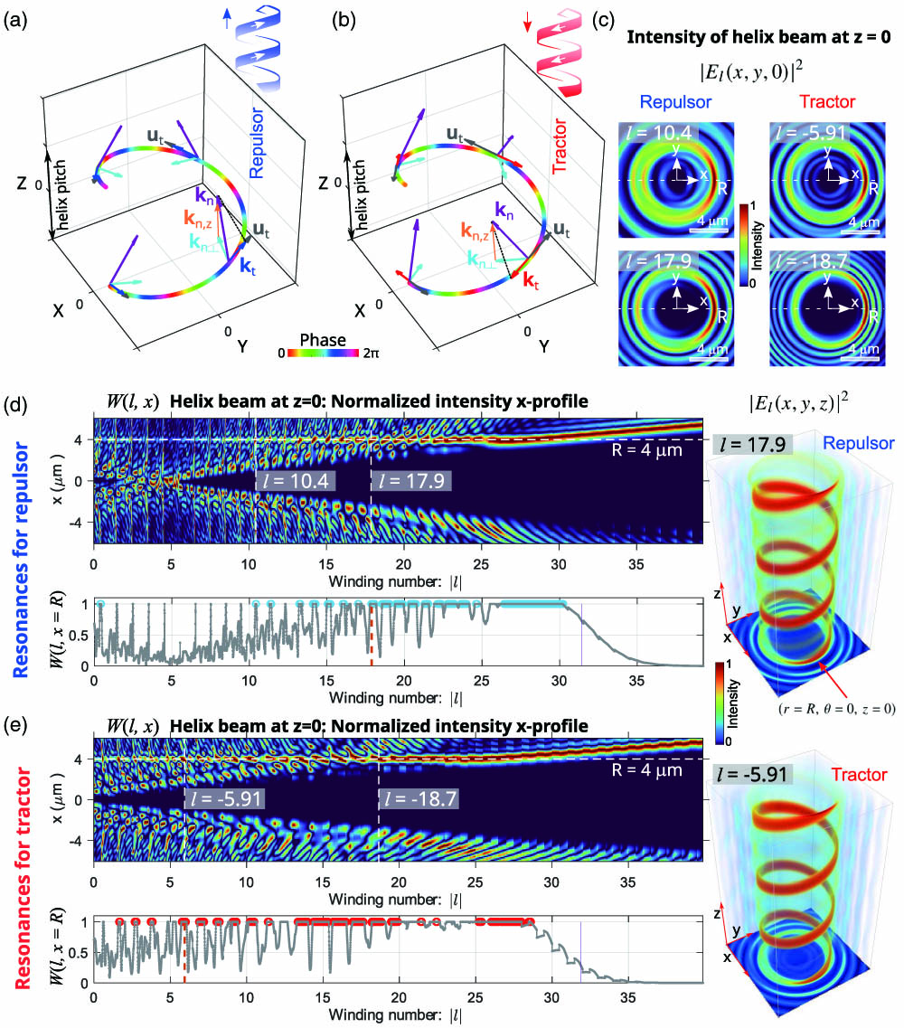
José A. Rodrigo*, Óscar Martínez-Matos, and Tatiana Alieva
Author Affiliations
  • Universidad Complutense de Madrid, Facultad de Ciencias Físicas, Ciudad Universitaria s/n, Madrid 28040, Spain
  • show less
    DOI: 10.1364/PRJ.468060 Cite this Article Set citation alerts
    José A. Rodrigo, Óscar Martínez-Matos, Tatiana Alieva. Helix-shaped tractor and repulsor beams enabling bidirectional optical transport of particles en masse[J]. Photonics Research, 2022, 10(11): 2560 Copy Citation Text show less
    Wave vector kn of one of the Bessel modes comprising a (a) repulsor and (b) tractor helix beam and its components k⊥n, kz,n, and kt are indicated along one helix loop. The phase gradient projection kt=utl/R2+γ2 on the helix does not depend on n, and it has the opposite direction for repulsor and tractor beams. (c) The intensity distributions |El(x,y,0)|2 of the repulsor and tractor helix beams corresponding to R=4 μm and pitch of 4.4 μm (γ>0) are displayed for several values of the resonant winding numbers l=lres as an example. The normalized intensity profiles W(l,x) of the beam Eq. (10), resulting from the resonance search algorithm, are displayed in (d) for the repulsor mode and (e) for the tractor one.
    Fig. 1. Wave vector kn of one of the Bessel modes comprising a (a) repulsor and (b) tractor helix beam and its components kn, kz,n, and kt are indicated along one helix loop. The phase gradient projection kt=utl/R2+γ2 on the helix does not depend on n, and it has the opposite direction for repulsor and tractor beams. (c) The intensity distributions |El(x,y,0)|2 of the repulsor and tractor helix beams corresponding to R=4  μm and pitch of 4.4 μm (γ>0) are displayed for several values of the resonant winding numbers l=lres as an example. The normalized intensity profiles W(l,x) of the beam Eq. (10), resulting from the resonance search algorithm, are displayed in (d) for the repulsor mode and (e) for the tractor one.
    Sketch of the experimental setup: optical trapping system (inverted widefield microscope and an SLM) and an optical scanning system [sCMOS camera and electrically tunable varifocal lens (ETL)] used for dynamic 3D imaging of the sample at a frame rate of 10 Hz. A collimated input laser beam (wavelength of λ0=1064 nm) illuminates the SLM, where the beam [Eq. (22)] has been encoded as a hologram. The encoded beam is projected (using the relay lens RL1 and the microscope’s tube lens, both with focal length of 200 mm) onto the back aperture of the objective lens (Nikon, 1.45 NA) that focuses the helix beam over the sample. The dynamic 3D image is reconstructed by a computer from the set of through-focus bright-field images collected by the scanning system. The achromatic relay lens RL2 has a focal length of 150 mm.
    Fig. 2. Sketch of the experimental setup: optical trapping system (inverted widefield microscope and an SLM) and an optical scanning system [sCMOS camera and electrically tunable varifocal lens (ETL)] used for dynamic 3D imaging of the sample at a frame rate of 10 Hz. A collimated input laser beam (wavelength of λ0=1064  nm) illuminates the SLM, where the beam [Eq. (22)] has been encoded as a hologram. The encoded beam is projected (using the relay lens RL1 and the microscope’s tube lens, both with focal length of 200 mm) onto the back aperture of the objective lens (Nikon, 1.45 NA) that focuses the helix beam over the sample. The dynamic 3D image is reconstructed by a computer from the set of through-focus bright-field images collected by the scanning system. The achromatic relay lens RL2 has a focal length of 150 mm.
    (a) Intensity and phase distributions of circular helix beams (radius R=4 μm, pitch of 4.4 μm) corresponding to (a) repulsor and (b) tractor modes for anticlockwise (γ>0) and clockwise (γ<0); see Visualization 1. The phase gradient projections along the helix of the repulsor (tractor) beam point downstream (upstream). These results correspond to the numerically propagated finite helix beam (axial extension Zeff=30 μm) calculated using Eqs. (3) and (22).
    Fig. 3. (a) Intensity and phase distributions of circular helix beams (radius R=4  μm, pitch of 4.4 μm) corresponding to (a) repulsor and (b) tractor modes for anticlockwise (γ>0) and clockwise (γ<0); see Visualization 1. The phase gradient projections along the helix of the repulsor (tractor) beam point downstream (upstream). These results correspond to the numerically propagated finite helix beam (axial extension Zeff=30  μm) calculated using Eqs. (3) and (22).
    (a) and (b) show volumetric representations (intensity values above the 75% of the maximum intensity) of a circular helix beam (R=4 μm and pitch of 4.4 μm) with axial extension of 30 μm and 12.5 μm, respectively. The third row displays the amplitude of the corresponding signals [Eq. (22)] encoded into the SLM. (c), (d) Volumetric representation of a triangular helix beam (pitch of 3.5 μm) with axial extension of 12.5 μm; see Visualization 2. (e) The extension of the circular helix beam has been estimated by using Eq. (21) for the cases (a) and (b), respectively.
    Fig. 4. (a) and (b) show volumetric representations (intensity values above the 75% of the maximum intensity) of a circular helix beam (R=4  μm and pitch of 4.4 μm) with axial extension of 30 μm and 12.5 μm, respectively. The third row displays the amplitude of the corresponding signals [Eq. (22)] encoded into the SLM. (c), (d) Volumetric representation of a triangular helix beam (pitch of 3.5 μm) with axial extension of 12.5 μm; see Visualization 2. (e) The extension of the circular helix beam has been estimated by using Eq. (21) for the cases (a) and (b), respectively.
    Experimental results. (a) Time lapse representation of the silica NP positions transported downstream during 6.8 s by a repulsor helix beam. (b) Time lapse representation of the NP positions transported upstream during 8.6 s by a tractor helix beam. (c) Time lapse representation of the NP positions during alternate bidirectional transport. Downstream and upstream transport has been sequentially applied in 5 cycles for a time of 16 s; see Visualization 3. The values of the axial position z of each NP are indicated in the color bar. The particle trajectory fits well to the experimental (d) repulsor and (e) tractor helix beams (volumetric intensity representation). (f) The corresponding transverse and axial intensity sections of the measured helix beams.
    Fig. 5. Experimental results. (a) Time lapse representation of the silica NP positions transported downstream during 6.8 s by a repulsor helix beam. (b) Time lapse representation of the NP positions transported upstream during 8.6 s by a tractor helix beam. (c) Time lapse representation of the NP positions during alternate bidirectional transport. Downstream and upstream transport has been sequentially applied in 5 cycles for a time of 16 s; see Visualization 3. The values of the axial position z of each NP are indicated in the color bar. The particle trajectory fits well to the experimental (d) repulsor and (e) tractor helix beams (volumetric intensity representation). (f) The corresponding transverse and axial intensity sections of the measured helix beams.
    Experimental results. (a) Time lapse representation of the positions and speed of the NPs transported downstream during 6.8 s by the repulsor helix beam. (b) Same time lapse representation for the NPs transported upstream during 8.6 s by the tractor helix. (c) Time lapse representation of the NP positions during alternate bidirectional transport. Downstream and upstream transport has been sequentially applied in five cycles for a time of 16 s; see Visualization 3. The histogram of NP speed values for each case is displayed in the second row. The third row displays the corresponding speed values given as a plot of the NP position z versus the polar angle θ, where the black dashed line corresponds to the helix curve. The NP trajectory fits well to the helix curve, and the NP speed values are mostly uniformly distributed along it.
    Fig. 6. Experimental results. (a) Time lapse representation of the positions and speed of the NPs transported downstream during 6.8 s by the repulsor helix beam. (b) Same time lapse representation for the NPs transported upstream during 8.6 s by the tractor helix. (c) Time lapse representation of the NP positions during alternate bidirectional transport. Downstream and upstream transport has been sequentially applied in five cycles for a time of 16 s; see Visualization 3. The histogram of NP speed values for each case is displayed in the second row. The third row displays the corresponding speed values given as a plot of the NP position z versus the polar angle θ, where the black dashed line corresponds to the helix curve. The NP trajectory fits well to the helix curve, and the NP speed values are mostly uniformly distributed along it.
    (a) Bright-field images of silica NPs transported along a circular and triangular helix, shown as an example. (b) The time lapse 3D image (time of 16 s) for each helix beam reveals the NPs optically trapped and transported along the helix as well as some of the free NPs. (c) A dynamic time lapse in 3D (for a lapse time of 2 s) is displayed for each case; see Visualization 3 and Visualization 4. (d) Measured intensity distributions of the repulsor and tractor triangular helix beams, displayed as volumetric representations along with transverse (x−y) and axial (y−z) sections.
    Fig. 7. (a) Bright-field images of silica NPs transported along a circular and triangular helix, shown as an example. (b) The time lapse 3D image (time of 16 s) for each helix beam reveals the NPs optically trapped and transported along the helix as well as some of the free NPs. (c) A dynamic time lapse in 3D (for a lapse time of 2 s) is displayed for each case; see Visualization 3 and Visualization 4. (d) Measured intensity distributions of the repulsor and tractor triangular helix beams, displayed as volumetric representations along with transverse (xy) and axial (yz) sections.
    Distribution of amplitude weights |n−l||Jn(k⊥nR)|/γ2 of the helical Bessel modes Jn(k⊥nr)exp[inϕ] comprising the beam described by Eq. (6) for a helix of radius R=4 μm and pitch of 2π|γ|=4.4 μm. The regions where repulsor and tractor beams can be found for γ>0 and γ<0 have been indicated as well. A zoom inset is also displayed to help the visualization.
    Fig. 8. Distribution of amplitude weights |nl||Jn(knR)|/γ2 of the helical Bessel modes Jn(knr)exp[inϕ] comprising the beam described by Eq. (6) for a helix of radius R=4  μm and pitch of 2π|γ|=4.4  μm. The regions where repulsor and tractor beams can be found for γ>0 and γ<0 have been indicated as well. A zoom inset is also displayed to help the visualization.
    The normalized intensity profile W(l,x) (as in the main text, Fig. 1) of the beam resulting from the resonance search algorithm is displayed in (a) and (b) for the repulsor and tractor modes (helix radius R=4 μm and helix pitch of 9.1 μm), respectively. The intensity distributions |El(x,y,0)|2 of the repulsor and tractor helix beams are also displayed for several values of the resonant winding numbers l=lres as an example.
    Fig. 9. The normalized intensity profile W(l,x) (as in the main text, Fig. 1) of the beam resulting from the resonance search algorithm is displayed in (a) and (b) for the repulsor and tractor modes (helix radius R=4  μm and helix pitch of 9.1 μm), respectively. The intensity distributions |El(x,y,0)|2 of the repulsor and tractor helix beams are also displayed for several values of the resonant winding numbers l=lres as an example.
    José A. Rodrigo, Óscar Martínez-Matos, Tatiana Alieva. Helix-shaped tractor and repulsor beams enabling bidirectional optical transport of particles en masse[J]. Photonics Research, 2022, 10(11): 2560
    Download Citation