Optical manipulation such as optical cooling, trapping, binding, and transporting of particles, has experienced intense development in the past three decades [1–6]. In the last decade, increasing attention has been devoted to mastering new techniques for optical transport and delivery of micro-objects even against the light propagation direction. Optical tractor beams, conceptually proposed in 2011 [7,8] and experimentally demonstrated in multiple works [9–16], offer the ability to pull particles against light propagation, which is interesting for optical transport. The reported optical tractor beams are based on different mechanisms to exert the required optical pulling force over the illuminated object, and most of them have relied on fine-tuning of the object material properties [12,15].

The so-called optical solenoid mode allows for the creation of a repulsor and tractor beam in the form of a helix as experimentally demonstrated in 2010 [9]. It can exert both pushing or pulling optical forces over the illuminated object which are responsible for downstream or upstream transport of the object along the solenoid [9], respectively. This has been achieved by an appropriately designed phase gradient [17] along the solenoid beam that redirects part of the light radiation pressure to create the required pushing or pulling optical force [18]. Note that the required retrograde (pulling) force arises when the illuminated particle scatters the wave’s momentum density downstream into the direction of light propagation and then it recoils upstream by conservation of momentum [18]. The phase-gradient-based mechanism allows switching between the repulsor and tractor beam just by reversing the phase gradient; thus, it enables a bidirectional optical transport along the solenoid beam [9]. This pioneering and visionary study did not receive the attention it merited. The only experimental demonstration of a solenoid tractor beam, applied for transport of a single dielectric micro-particle (silica sphere of 1.5 μm in diameter) along a part of the circular helix turn, has been reported in Ref. [9]. However, it remains unclear whether the solenoid beam can simultaneously transport multiple particles or be not along multiple loops of the helix, which in turn is a crucial requisite for practical optical transport applications.

Non-diffracting beams [19,20] are promising for generating tractor beams because they can maintain both intensity and shape in the propagation direction, which is essential for long-range particle transportation. The solenoid beam belongs to the family of the non-diffracting rotating beams [19,20]; therefore, it would provide long-range transportation. However, it corresponds to the ideal solution of a helix beam of infinite axial extension, which is not physically realizable. Other proposed tractor beams [7,8,10–16] are also limited by the axial extension of the beam.

Here, we get back to the important problem of the design and creation of phase-gradient-based repulsor and tractor helix-shaped beams suited for bidirectional optical transport of multiple particles along a three-dimensional (3D) trajectory. Our approach is based on the so-called polymorphic beam, which is a kind of structured laser beam whose intensity and phase gradient forces can be independently prescribed along an arbitrary 3D trajectory to drive the optical transport of particles along it; see, for example, Refs. [21–23].

The goal of this work is twofold: first, to present and clarify crucial aspects of the theory required for the design and correct experimental generation of helix-shaped repulsor and tractor beams displaying discrete propagation invariance and, second, to experimentally study the optical transport of particles driven by helix beams of different geometry. We report the first experimental evidence of simultaneous transport of multiple particles along multiple loops of the helix beam, which underlines its inherent structural robustness in the presence of multiple particles. This robustness of the helix-shaped beams allows us to study the bidirectional 3D optical transport of particles en masse along the same helix as an exploring test previous to future applications.

The work is organized as follows. Section 2 introduces the theoretical background and establishes the design rules of helix beams with infinite axial extension, underlying the crucial role played by the resonance-like selection of the phase gradient that governs the helix beam creation, and Section 3 is devoted to physically realizable helix beams with finite axial extension. The analytical expressions that describe the design of such a finite helix beam as well as predict its axial extension are presented. The reduced axial extension is due to the limitations of the optical system required for the experimental generation of the helix beam. Section 4 presents an analysis of the experimental results that demonstrate the performance of the considered helix-shaped beams for simultaneous optical transport of multiple dielectric nanoparticles (NPs, silica sphere of 500 nm in diameter). The work ends with concluding remarks and discussions.

Let us first briefly revise a direct method for 3D laser curve generation based on the polymorphic beam approach. A coherent polymorphic laser beam [21–23] can be transformed around the focal plane (e.g., at z=0) of an objective lens into a 3D light curve represented by c(t)=(R(t),Z(t)), with R(t)=(R(t)cost,R(t)sint). Its intensity and phase distributions can be independently controlled along the curve [21,22,24]. Specifically, the angular spectrum A0(k⊥,z) of a polymorphic beam at z=0 is defined as follows: A0(k⊥,0)=∫−∞∞g(t)exp[−iZ(t)k2−k⊥2]exp[ik⊥R(t)]dt.(1)Here, k=2π/λ is the wavenumber with wavelength λ in the mounting medium where the laser beam is focused, and k⊥=(kx,ky) is the projection of the wave vector k on the transverse plane (perpendicular to the optical axis). The expression Eq. (1) is reduced to the paraxial form reported in Refs. [21–24]. Here, g(t) is a complex-valued weight that plays an important role in the design of the complex amplitude of the laser curve described by c(t). Specifically, the modulus |g(t)| (in units V m) defines the intensity distribution along the curve and its length. For instance, the intensity distribution is uniform along the curve if |g(t)|∝|c′(t)|, where c′(t)=dc(t)/dt=(R′(t),Z′(t)). The length of the curve can be reduced by using |g(t)|→|g(t)|rect(t/T), where the parameter T stands for the maximum value of the polar angle (e.g., t) parametrizing the curve. The phase along the curve is given by Ψ(t)=arg[g(t)], and it can be defined as Ψ(t)=2πL·S(t)/S(T). Therefore, the phase distribution is uniform along the curve when S(t)=∫0t|c′(τ)|dτ. The term 2πL is the phase accumulation along the curve with L being a real number [25]. Further information about the phase design along the curve has been reported in Ref. [22].

Since the expression Eq. (1) corresponds to the angular spectrum of the polymorphic beam at the focal plane of the objective lens (corresponding to the position z=0), one can write the angular spectrum for any value of z as [26] A0(k⊥,z)=A0(k⊥,0)exp(izk2−k⊥2),(2)as well as for the corresponding complex field amplitude in the focusing region where the light curve is created: E(r,z)=14π2∫−kkA0(k⊥,0)exp(izk2−k⊥2)exp(−irk⊥)dk⊥.(3)

Thus, there is a direct relation between the Eq. (1) and the field amplitude projected on the back focal plane of the Fourier transforming lens applied to create the light curve. Further, only the transmitted wave (k2>k⊥2) will be considered.

In the case of curves with rotational symmetry, it is often useful to rewrite Eqs. (1) and (3) in cylindrical coordinates k⊥=(k⊥,ϕ) and r=(r,θ) as follows: A0(k⊥,ϕ,0)=∑n=−∞∞inexp(inϕ)∫−∞∞g(t)exp[−iZ(t)k2−k⊥2]⁢Jn[k⊥R(t)]exp(−int)dt,(4)E(r,θ,z)=14π2∫0k∫02πk⊥A0(k⊥,ϕ,0)exp(izk2−k⊥2)⁢exp[−irk⊥cos(ϕ−θ)]dk⊥dϕ,(5)where the indices n are integer numbers. The considered expressions can be applied for arbitrary curves. Here, we are interested in helices for the generation of helix-shaped beams working as repulsor or tractor beams. The design and main properties of such beams are considered in the next sections.

Let us first consider a circular helix of constant radius R, curvature, and torsion. It is described in Cartesian coordinates as c(t)=(Rcost,Rsint,tγ), with 2π|γ| being the helix pitch (height of one complete helix loop). Note that the sign of γ=Rtanβ (where β is the helix slope angle) defines the chirality of the helix. It is right-handed (counter-clockwise rotation) when γ>0 and left-handed (clockwise rotation) for γ<0. For the case of a circular helix, the expression |c′(t)|=R2+γ2 holds, and a uniform intensity and phase distributions are prescribed along it by using g(t)=g0exp(ilt), where 2πl is the phase accumulation over a complete helix loop. Thus, the phase of the helix beam can be tuned by means of the winding number l. By introducing g(t)=g0exp(ilt) in Eq. (4), the following expression for the angular spectrum of a circular helix beam is obtained: $$\begin{gathered} A0(k⊥,ϕ,0)=g0∑n=−∞∞inJn(k⊥R)exp(inϕ)⁢∫−∞∞exp[i(l−n)t]exp(−itγk2−k⊥2)dt \\ =2πg0∑n=−∞∞inJn(k⊥R)exp(inϕ)δ(l−n−γk2−k⊥2) \\ =2πg0γ2∑n∈Ωin|l−n|k⊥nJn(k⊥nnR)exp(inϕ)δ(k⊥−k⊥n), \end{gathered}$$(6)where Ω is a set of the allowed Bessel mode with indices n defined further and k⊥n=k2−(l−n)2γ2.(7)

It is not surprising that the expression Eq. (6) is a combination of concentric Montgomery rings [defined by δ(k⊥−k⊥n)], which describe the angular spectrum of rotating [27] and more general self-imaging beams [28]. The circular helix is a particular case of the family of rotating beams [27] whose complex field amplitude satisfies the condition Erot(r,θ±kγ,z+2πγ)=exp[iζ(r,θ,γ)]Erot(r,θ,z), where ζ(r,θ,γ) is an arbitrary real function whereas γ also defines both the direction of rotation and the value of the longitudinal period of the field. It is a set of concentric rings whose amplitudes and radii k⊥n define the shape of the rotating beam [27]. In particular, the radius R of the circular helix beam is determined only by the complex-valued amplitudes of Montgomery rings of radii k⊥n given by Eq. (7).

The set Ω of Bessel mode indices applied in Eq. (6) is defined by the conditions k2≥(l−n)2/γ2 and kz=(l−n)/γ>0. Therefore, this set depends on wavenumber k, winding number l, and helix pitch 2π|γ|. For positive γ (right-handed helix), the set Ω is settled as γ>0,l−γk<n<l.(8)

One can observe that when the value of the index n increases then k⊥n decreases. However, when |n| increases, k⊥n decreases; therefore, the radius of the Montgomery ring decreases for positive l (repulsor beam), while k⊥n increases for negative l (tractor beam). Correspondingly, for negative γ (left-handed helix), the set Ω is written as γ<0,l<n<l−γk.(9)

In this case, when n increases, then k⊥n increases. Note that when |n| increases k⊥n increases for positive l (tractor beam) and decreases for negative l (repulsor beam). Thus, one can see that for a given value of l the Montgomery rings with the largest radius always correspond to the largest allowed index |n| for the tractor beam and the smallest index |n| for the repulsor one. This fact is important for the experimental implementation of the helix beam (Section 3) due to the limited aperture of the optical setup. Note that in the case of the tractor beam the Bessel mode indices n have always the same sign as γ, whereas for the repulsor beam the indices n can have the same, opposite, or even mixed signs depending on the value of l (see Appendix A).

Let us recall that the Fourier transform of inexp(inϕ)·δ(k⊥−k⊥n)/k⊥ is a helical Bessel mode Hn(k⊥nr,ϕ)=Jn(k⊥nr)exp(inϕ) [29]. Then the circular helix beam is the superposition of certain helical Bessel modes. According to Eq. (2), the evolution of a helical Bessel mode during propagation is described as Hn(k⊥nr,ϕ)exp(izk2−k⊥2)=Hn(k⊥nr,ϕ)exp[iz(l−n)/γ]. Thus, one obtains the following expression for the infinite (ideal) circular helix beam: E(r,θ,z)=g0γ2exp(izlγ)∑n∈Ω|l−n|Jn(k⊥nR)Jn(k⊥nr)⁢exp[in(θ−zγ)],(10)around the focal plane (at z=0) of the Fourier transforming lens, where the indices n satisfy Eq. (8) or Eq. (9) for right- or left-handed helices, respectively. Note that the same expression Eq. (10) has been also found in Ref. [9] to describe the solenoid beam.

However, the expressions Eqs. (8)–(10) are necessary but not sufficient conditions for the creation of a helix-shaped light curve. Let us analyze these equations and identify their important limitations. One can see that the phase accumulation is 2πl along a helix pitch 2π|γ|, as it has been prescribed. Moreover, the phase gradient ∇Ψ|r=R of the beam E(R,θ,z) projected onto the helix is given by kt=utl/R2+γ2, where ut is a unit vector tangent to the helix, and it is defined in Cartesian coordinates as ut=1R2+γ2(−Rsinθux+Rcosθuy+γuz).(11)

Indeed, the gradient of the phase Ψn=(l−n)z/γ+nθ of any Bessel mode (of the set Ω) evaluated at r=R is written as ∇Ψn|r=R=−nRsinθux+nRcosθuy+(l−n)γuz.(12)

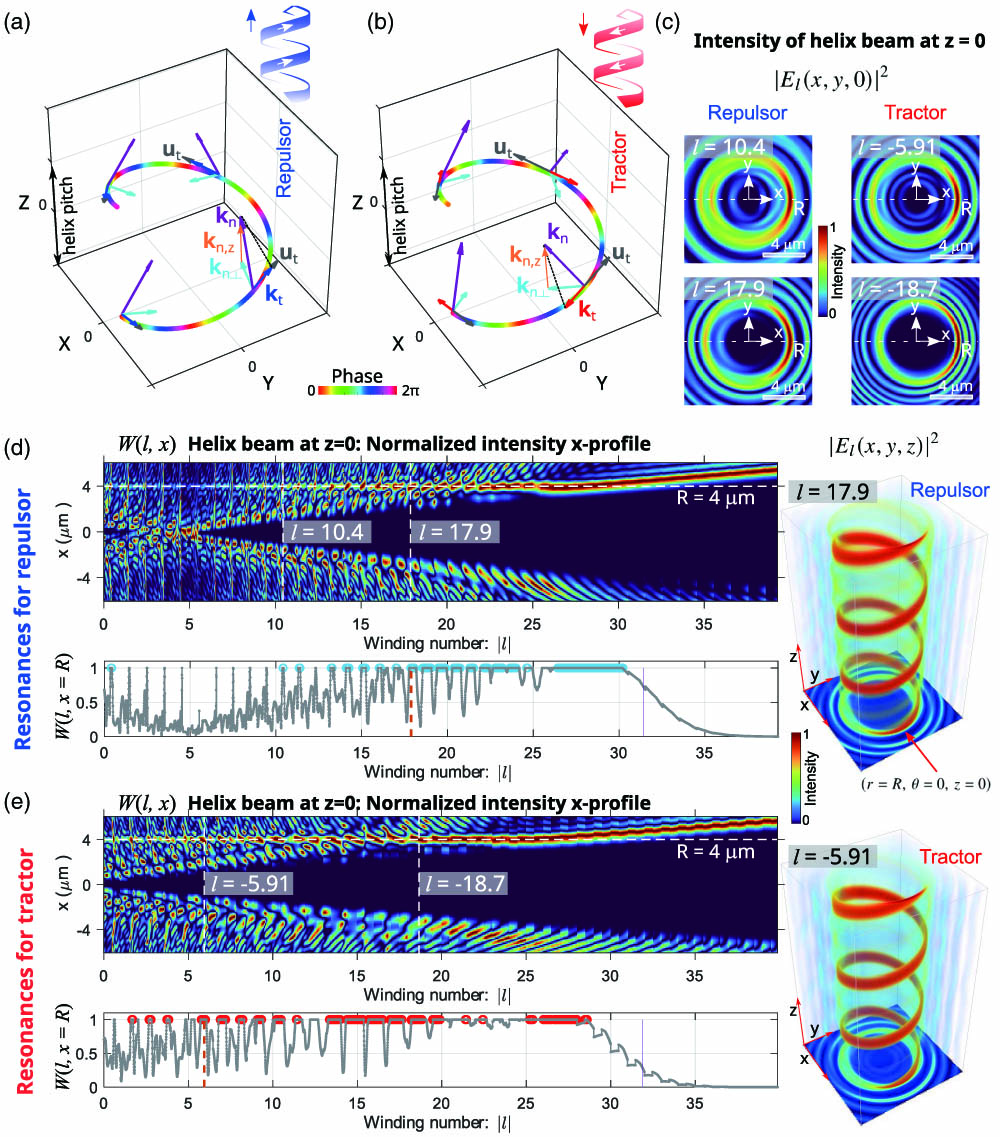
Thus, all the Bessel modes of the set Ω have the same phase gradient projection given by ξt=ut∇Ψn|R=l/R2+γ2, at any point with radial coordinate r=R. In Fig. 1, the projections of the wave vector kn of one of the modes (n∈Ω) comprising the helix beam are shown. For both repulsor and tractor beams [see Figs. 1(a) and 1(b)], the wave vector component kn,z is always pointing into the light propagation direction (i.e., along the z axis), and the component kt is pointing in the same and opposite direction to the tangent vector ut for repulsor and tractor, respectively. Because the value of |kt|=kt has to be less than k, there exists a limitation for the maximum value of the winding number: |l|<|lmax|=kR2+γ2. Moreover, this limitation is even more restrictive for tractor helix beams: |l|<|lmax|=kR. Indeed, since kz>0, then kt<k⊥=kR/R2+γ2 and, therefore, |l|<kR for tractor helix beams.

In addition, only certain values of the winding number l allow the creation of a helix beam with the prescribed radius R, helix pitch 2π|γ|, and wavenumber k. This important constraint for the winding number arises from the behavior of both the Bessel modes Jn(k⊥nr) and their weights w(n∈Ω,l,γ)=|n−l|Jn(k⊥nR)exp(inθ) describing the beam Eq. (10). Specifically, a helix beam can be only created when the constructive interference of the modes w(n∈Ω,l,γ)Jn(k⊥nr) yields the maximum of the intensity distribution |El(r,θ,z)|2 at the point (r=R,θ=z/γ,z). This is only possible for certain values l=lres, which in this context will be further referred to as resonant winding numbers. Let us recall that the function k⊥n also depends on the winding number l [see Eq. (7)], and then it also plays a role in the resonance through the function Jn(k⊥nr). Let us underline that a helix beam might be created with at least two Bessel modes; thus, k|γ|≥2, which means that the helix pitch has to be larger than 2λ. Note that in the case of a solenoid beam (circular helix) comprising the superposition of only two Bessel modes the value of l can be found by using the optimized interference condition proposed in Ref. [18].

To find the resonant values lres, the following resonance search algorithm can be applied. This algorithm consists of the analysis of the intensity distribution |El(r,θ,z)|2 for only one transverse plane, for example at z=0, due to the beam symmetry. The first step is to verify that the global intensity maximum (i.e., the peak intensity) is located at the expected helix point (r=R,θ=0,0). The second step is to check that the local maxima are below a chosen threshold, for example, a ∼70% of the peak intensity. This resonance search algorithm has been implemented in a program for automatic and fast search of l=lres of the helix beams. To illustrate its performance, let us consider a helix with radius R=4μm and pitch of 4.4 μm (γ>0) corresponding to a helix slope angle β=10°, whereas the light wavelength is λ=800nm in the medium (water, as in our experiments). The intensity distributions |El(x,y,0)|2 of the corresponding repulsor and tractor helix beams are displayed in Fig. 1(c) for different values of lres. The normalized intensity profile W(l,x)=|El(x,y=0,z=0)|2/max{|El(x,y,0)|2} of the beam along the x–axis is displayed as a function of the winding number l for this helix, for both repulsor [Fig. 1(d)] and tractor [Fig. 1(e)] modes. In this map for W(l,x), it is observed that only certain values of the winding number l yield a peak intensity at the point x=R of the helix. The values of W(l,x=R) are also displayed for each case where the resonant values lres are indicated by blue and red circles for repulsor and tractor helix beams, correspondingly. Let us underline that the value of the winding number is limited by |lmax|=kR2+γ2=32 and |lmax|=kR=31.4 for the considered repulsor and tractor helix beams, respectively. As observed in Figs. 1(d) and 1(e), the radius of the helix beam coincides with the expected one R=4μm for values |lres|<lmax. For instance, the resonant values lres=17.9 and lres=−5.91 correspond to the repulsor (with phase gradient projection ξt=4.4μm−1) and tractor (with ξt=−1.46μm−1) helix beam whose intensity distribution |El(x,y,z)|2 is displayed as a volumetric representation in Figs. 1(d) and 1(e) as well. The intensity values above ∼70% of the peak intensity correspond to the prescribed helix as expected. Interestingly, for values |l|>lmax, a helix beam with increasing radius can be created as observed in the map W(l,x) displayed in Figs. 1(d) and 1(e). Nevertheless, in this forbidden region above lmax, the beam Eq. (10) rapidly collapses to a single Bessel mode with index n→l.

The existence of resonances for a helix beam and the limits of its winding number have not been previously reported. The knowledge of these resonances is crucial for the creation of helix-shaped repulsor and tractor beams providing a new insight into their behavior. Moreover, it underlines that only certain values of the phase gradient projection ξt=lres/R2+γ2, which defines the propulsion force exerted by a repulsor and tractor helix beam, can be prescribed. The described resonance search algorithm provides the allowed winding numbers lres, and it has been applied for the creation of the helix beams considered in this work. Note that for helix beams with γ>0 the tractor and repulsor case corresponds to ξt<0 and ξt>0, respectively. Thus, the particle can be transported downstream for ξt>0 and upstream for ξt<0 along a right-handed helix (γ>0), and vice versa for a left-handed helix (γ<0).

The dipole approximation (corresponding to a Rayleigh particle of radius a<0.1λ) provides a straightforward interpretation of the confinement and propulsion forces as a function of the beam intensity and phase distributions [4,18]. Note that the light polarization plays a little role in the electric dipole force at first order [4,18], which is our case. A detailed theoretical analysis of the optical forces exerted by tractor beams in the Rayleigh limit for first and higher orders, including solenoidal tractor beam modes, has been reported in Ref. [18]. As a rule of thumb, it is often assumed, as a reasonably good approximation, that the optical propulsion force F arising from the radiation pressure is proportional to the product of the beam intensity I and phase gradient ξt as follows: F=σextIξtut/ck0 [23]. Here, σext is the extinction cross section of the particle, which can be numerically calculated by using the well-known Mie scattering theory for slightly larger particles [30]. Note that if the radius R or the helix pitch 2π|γ| is changed the strength of the propulsion force |F|∝I·lres/R2+γ2 is also changed, which can alter the particle transport efficiency. Moreover, let us recall that the helix pitch has to be larger than 2λ, which also sets a limit to the minimum value of R for a fixed value of the helix slope.

Let us now consider how to create a generalized helix beam whose shape, intensity, and/or phase distributions can be non-uniform along the helix if needed. Such a generalized helix beam is described by the curve c(t)=(R(t)cost,R(t)sint,tγ), with 2π|γ| being the helix pitch. This kind of generalized helix beam belongs to the class of self-imaging beams that satisfy the following condition: Es−im(r,θ,z+2πγ)=exp(iζ)Es−im(r,θ,z). Montgomery demonstrated that these beams can be also presented as a linear superposition of Bessel modes [28]. Thus, our goal is to define the coefficients of these Bessel modes to construct a generalized helix beam with independent control of its shape c(t), intensity, and phase distributions.

We return to the general expression for the polymorphic beam written in polar coordinates, Eq. (4). Since the helix is a periodic curve in the axial direction z, then g(t)Jn[k⊥R(t)] can be represented as a Fourier series, g(t)Jn[k⊥R(t)]=∑m=−∞∞am,n(k⊥)exp(imt),(13)where am,n(k⊥)=12π∫−ππg(τ)Jn[k⊥R(τ)]exp(−imτ)dτ.(14)

By introducing Eq. (13) into Eq. (4), the angular spectrum expression in the form of a combination of the Montgomery rings is again obtained: A0(k⊥,ϕ,0)=2π∑m=−∞∞∑n=−∞∞inexp(inϕ)am,n(k⊥)⁢δ(m−n−γk2−k⊥2).(15)

The analysis of the argument of δ-function shows that the same selection rules (defining the set Ω of allowed indices n) as in Eq. (7) and in Eqs. (8) and (9) hold for k⊥ and for the indices n, correspondingly, if one substitutes l by m. Thus, we obtain A0(k⊥,ϕ)=2πγ2∑n∈Ωinexp(inϕ)∑m=−∞∞|m−n|k⊥am,n(k⊥n)δ(k⊥−k⊥),(16)where k⊥n=k2−(m−n)2γ2.(17)

Note that the allowed values of m are defined by the expression Eq. (14). By following a similar approach to the one considered in Section 2.B, the focused helix beam around the focal plane can be written as E(r,θ,z)=2πγ2∑n∈Ωexp(inθ)⁢∑m=−∞∞|m−n|am,n(k⊥n)Jn(k⊥nr)exp(izm−nγ).(18)

The same selection rules (defining the set Ω of allowed indices n) as in Eq. (7) and in Eqs. (8) and (9) hold for k⊥n and for the indices n, correspondingly, if one substitutes l by m. The choice of transmitted Bessel modes depends on the values of am,n(k⊥n), where |m−n|≤|γ|k and (m−n)/γ>0, which again proves that an arbitrary configuration of the helix beam is not possible.

For a helix beam with a uniform phase and amplitude distribution along the curve, the term an,m(k⊥) is given by am,n(k⊥)=g02π|c′(2π)|∫−ππ|c′(τ)|⁢exp[il∫0τ|c′(s)|ds|c′(2π)|]Jn[k⊥R(τ)]exp(−imτ)dτ,(19)where |c′(τ)|={[R(τ)]2+[R′(τ)]2+[Z′(τ)]2}1/2.

In particular, for the case of the circular helix with uniform amplitude and phase distribution along the helix, only one term m=l in the decomposition Eq. (13) is allowed: am,n(k⊥)=g0Jn(k⊥R)δm,l. However, if the phase distribution of the circular helix is not uniform, for example, g(τ)=g0exp[i(lτ+bsinτ)], then the coefficients are am,n(k⊥)=g0Jn(k⊥R)Jm−l(b), where we have considered integer l. As in the case of the circular helix beam studied in the previous section, the resonance search algorithm can be also applied to find the resonant winding numbers lres for the case of the generalized helix beam.

Helices shaped in different forms can be easily created with the radius R(t)=ρ[|1acos(M4t)|n2+|1bsin(M4t)|n3]−1/n1,(20)which corresponds to the Superformula [31] often used for modeling abstract and natural shapes. The set of real numbers Q=(ρ,a,b,n1,n2,n3,M) in Eq. (20) allows the generation of a wide variety of shapes of different symmetry. For instance, the set Q=(R,1,1,6,6,6,3) allows the generation of the triangular helix considered in the next sections.

In the previous section, we have established the construction rules for the infinite helix beam of different chirality, shape, and winding number l. However, there is no optical system able to generate an ideal helix beam of infinite extension. Thus, the design of a physically realizable helix beam requires taking into account the characteristics and limitations of the optical system that, in particular, reduces the helix extension. Basically, the generation of a helix beam requires a coherent laser beam and an optical system comprising a spatial light modulator (SLM) device for encoding the polymorphic beam as well as a focusing objective lens with focal length f and numerical aperture NA, as sketched in Fig. 2.

The SLM is a programmable device that allows the holographic encoding [32] of a complex field amplitude E0(r0) given by Eq. (1) [or Eq. (4)] in our case. Note that k⊥=kr0/f2+r02, where r0=(x0,y0) is the spatial coordinates in the SLM plane (display) [19]. The main limitation of an SLM is its pixelated display, whose spatial resolution is typically limited by a micron-sized pixel. A Montgomery ring modulated by the corresponding helical phase [see Eq. (6)] can be represented in practice as a ring of width dn corresponding to several pixels. This limitation is responsible for the finite axial extension Zeff of the helix beam.

To estimate the axial extension Zeff of the helix, we have considered the degradation of a helical Bessel mode exp(inϕ)Jn(k⊥r) generated by a Montgomery ring of radius rn and width dn using the Fourier transforming property of a focusing lens. Specifically, by generalizing the approach reported in Ref. [33] (for the estimation of the Bessel J0-beam intensity degradation along the optical axis) to a helical Bessel mode, we have obtained the following expression: In(R,z)∝|∫ζ1ζ2Jn(kR1−ζ2)exp(ikzζ)ζdζ|2,(21)which describes the intensity evolution of the helix beam along the z direction at the point r=R, where integration limits are ζ1,2=f/f2+(r0,n±dn/2)2. The value of Zeff where the intensity In(R,z) of one of the transmitted Bessel modes decreases by a ratio of 25% (following a Rayleigh criteria) can be considered as the effective length of the helix beam. Note that integration limits ζ1,2 are given as a function of the Montgomery ring parameters (its radius r0,n and width dn) as well as of the focal length f of the objective lens. Thus, the effective length (extension) of the helix beam also depends on the value of this focal length.

The expression for the complex field amplitude corresponding to a finite circular helix beam (encoded into the SLM), E0(r0,ϕ)∝g0T∑n=−∞∞inexp(inϕ)Jn(kr0f2+r02R)⁢sinc[(l−n−γkff2+r02)T2],(22)can be easily derived from Eq. (6) by using |g(t)|=g0rect(t/T), where sinc(x)=sinx/x and T=Zeff/|γ| account for the axial extension Zeff of the helix beam. Note that the beam E0(r0,ϕ), Eq. (22), is optically projected (by using a 1× Keplerian telescope comprising two relay lenses, RL1 in Fig. 2) onto the back aperture plane (entrance pupil) of the objective lens, which focuses it in the form of a helix over the sample (in the mounting medium).

Let us underline that the sinc(·) function in the expression Eq. (22), corresponding to the finite circular helix, reaches its maximum value at the same position r0,n of the nth Montgomery ring defined by the delta function δ(k⊥−k⊥n) in Eq. (6) for the infinite circular helix. Thus, the sinc(·) functions replace the Montgomery rings comprising the field E0(r0,ϕ). Moreover, the indices n in the summation Eq. (22) follow the same selection rule given by Eq. (8) for γ>0 and Eq. (9) for γ<0.

Another important limitation arises from the characteristics of the objective lens. According to the specifications of the microscope objective manufacturer, the radius of the entrance pupil of an objective is given by r0,max=fNA. We recall that the numerical aperture of the immersion objectives lens is NA=nimmsinα, where nimm is the refractive index of the immersion medium. Thus, the maximum transverse projection of the wavenumber k of the laser beam before entering in the mounting medium is k⊥,maximm=k0NA=k0nimmsinαimm. In practice, the condition NA≥nm holds for oil immersion objectives, and the maximum transverse projection k⊥,maxm=k0nm<k⊥,maximm corresponds to the laser beam (e.g., the helix beam) focused in the mounting medium of refractive index nm. This constraint is derived from the Snell law nimmsinαimm=nmsinαm due to the focusing angle limitation corresponding to the total internal reflection on the glass-water interface of the sample. It means that the effective entrance pupil radius is r0,maxeff=fnm when NA≥nm. Since E0(r0,ϕ) is optically projected onto the objective’s back aperture, then only the Montgomery rings with radius r0,n<r0,maxeff can be transmitted through the objective and then participate in the formation of the focused helix laser beam.

In the case of a dry objective lens, the conditions NA<nm and r0,n<r0,max=fNA hold; however, when k⊥,maxm=k0NA<k0nm, then the mode index selection rule [given by expressions Eqs. (8) and (9)] has to be corrected as follows: $$\begin{gathered} γ>0,l−γk0nm2−NA2<n<l, \\ γ<0,l<n<l−γk0nm2−NA2. \end{gathered}$$(23)

This indicates that k0|γ|(nm−nm2−NA2)≥2 has also to be fulfilled for the transmission of at least two Bessel modes when NA<nm. These constraints dictate a threshold for the value of the helix pitch for each case: 2π|γ|≥{2λ0/nm,ifNA≥nm2λ0/(nm−nm2−NA2),ifNA<nm.(24)

Let us recall that the described resonance search algorithm providing the resonant winding numbers lres can be also applied for the finite circular helix [Eq. (22)]. The finite helix beam is created if a sufficient number of modes with k⊥n(lres)<k⊥,maximm can be transmitted through the optical system. Depending on the considered optical system, this constraint can be very restrictive; therefore, the design parameters of the helix beam (its radius R, γ, and lres) have to be properly chosen to allow the transmission of a sufficient number of modes.

Volumetric representations of the intensity and phase distributions of a finite helix beam with radius R=4μm and pitch of 4.4 μm, corresponding to the case NA≥nm (as for the infinite helix Fig. 1), are displayed in Fig. 3 for different helix handedness and values of the winding number l. They have been created by introducing the expression Eq. (22) of the polymorphic beam into the expression Eq. (3) and computing the beam propagation (using experimental parameters provided in the next section) for a range of 30 μm around the focal plane of the objective lens. Irrespective of the handedness of the helix [see Figs. 3(a) and 3(b), with γ>0 and γ<0 for right- and left-handed, respectively], a uniform phase distribution is observed along the curve for both tractor and repulsor configurations as prescribed.

To help the 3D visualization of the beam intensity distribution, only the values above the ∼75% of its peak intensity (maximum) are displayed in Figs. 4(a)–4(c), which corresponds to the intensity threshold used for the estimation of Zeff. The intensity distributions of the same circular helix beam (tractor with R=4μm, pitch of 4.4 μm, and l=−5.91) with Zeff=30μm and Zeff=12.5μm are shown in Figs. 4(a) and 4(b), respectively. The considered triangular helix beam [given by Eq. (20) with Q=(4μm,1,1,6,6,6,3), pitch of 3.5 μm, and l=−5.45] displayed in Figs. 4(c) and 4(d) has an axial extension of Zeff=12.5μm.

The axial extension Zeff of the numerically propagated circular helix beams [Figs. 4(a) and 4(b)] coincides with the estimated one obtained by computing the integral Eq. (21) for different values of the propagation distance z [see Fig. 4(e)]. Specifically, the estimated value of Zeff has been obtained from the normalized intensity profile In(R,z)/In(R,0) for each case, where n=−11 is the index of the Bessel mode associated with the wider Montgomery ring of the set comprising the tractor helix beam (l=−5.91) of this example. The set of Montgomery rings transmitted by our objective lens (with r0,maxeff=2.66mm) is also displayed in the third row of Figs. 4(a) and 4(b), and they have the following radius: r0,n=−10=1.86mm and r0,n=−11=0.89mm. The widest Montgomery ring has a width dn=−11=96μm (a size of ∼10 pixels of our SLM) and dn=−11=250μm for each case, in Figs. 4(a) and 4(b), respectively. Note that in Fig. 4(e) the intensity profiles In=−11(R,z)/In=−11(R,0) have been represented for each case along with a green line indicating the 75% intensity threshold used for the estimation of Zeff.

Wider Montgomery rings allow the focus of more light into the helix beam, which makes it easier to achieve stable optical trapping and transport of particles along it. Nevertheless, it would significantly decrease the axial extension Zeff of the helix beam.

As previously mentioned, the helix-shaped laser beam is created by using the experimental setup sketched in Fig. 2 comprising a near-infrared laser, an inverted bright-field microscope, and a programmable SLM used for holographic beam shaping. Specifically, the complex field amplitude given by Eq. (22) has been encoded onto the SLM (reflective phase-only SLM-liquid crystal on silicon, Meadowlark Optics, HSP1920-600-1300-HSP8, 8-bit phase level, pixel size of 9.2 μm) as a phase-only hologram by using a well-known encoding technique [32]. The SLM modulates the input collimated infrared laser beam (Azurlight Systems, ALS-IR-1064-10-I-CP-SF, λ0=1064nm, maximum optical power of 10 W, power stability <±0.3%, pointing stability <±0.5μrad/°C, linearly polarized), which is then optically projected (by the 1× Keplerian telescope comprising the microscope tube lens and a relay lens RL1 as indicated in Fig. 2) onto the back aperture of the microscope objective lens (Nikon CFI Plan Apochromat Lambda 100×, 1.45 NA, focal length f=2mm, and oil immersion nimm=1.512). The laser beam has been circularly polarized by using a quarter-wave plate for proper focusing of the trapping beam.

Our experimental setup also comprises a high-speed optical scanning system (OSS, see Fig. 2), enabling in situ dynamic 3D visualization of the sample almost in real time, as reported in Ref. [34]. This OSS consists of a scientific Complementary Metal-Oxide-Semiconductor (sCMOS) camera (Hamamatsu, Orca Flash 4.0, 16-bit gray-level, pixel size of 6.5 μm, operating at 500 Hz with an exposure time of 1 ms) and an electrically tunable lens (ETL, Optotune EL-10-30-C) mounted in front of the camera (see Ref. [34]). The ETL is a programmable varifocal lens that allows for high-speed optical scanning of the sample without the need of mechanical axial movement of the microscope sample stage. Here, we have used the OSS to measure multiple stacks of bright-field images required for a video-rate 3D visualization (10 Hz) of the experiments. Each stack has been measured in a time of 50 ms and corresponds to a volume of 20μm×20μm×8μm of the sample, which is enough for dynamic 3D visualization of the considered optical transport experiments. Nevertheless, faster video-rate 3D visualization (e.g., at 30 Hz) is possible just by using a high-speed sCMOS camera in the OSS [34].

Here, we have used silica nano-spheres (Sphero Tech) of radius a=250nm to study their transport driven by tractor and repulsor helix-shaped laser beams with radius R=4μm and pitch of 3.5 μm. In the experiment, the laser power measured at the back aperture of the objective lens is 360 mW and 330 mW for the repulsor and tractor helix beams, respectively. The considered dielectric NPs have been dispersed in aqueous solution (water, nm=1.33), and the sample has been sandwiched between two glass coverslips (#1.5H, 170±5μm thickness, Thorlabs CG15KH1) separated by a spacer ∼100μm thick.

To analyze the behavior of the repulsor and tractor helix-shaped beams, we performed 3D particle tracking for each measured stack of bright-field images recorded by the sCMOS camera of the OSS. We have used the open source particle tracking software reported in Ref. [35]. The tracking software provides both the particle position and speed data for each time value. It has been used to develop a program to analyze and visualize in 3D the tracking data as it is displayed in Figs. 5 and 6 for the particle position and speed, respectively. A mean number of 28 particles have been simultaneously transported along the helix trap for a time of 16 s.

The positions of all the tracked particles reveal the helix shape of the repulsor and tractor beams as observed in Figs. 5(a) and 5(b), respectively. These results confirm the stable confinement of the particles optically transported along the circular helix beam trap, downstream in Fig. 5(a) and upstream in Fig. 5(b). Note that in the experiment the repulsor and tractor beams have been switched each 2 s for alternating the optical transport between downstream and upstream transport (see Visualization 3). The particle positions observed in Fig. 5(c) correspond to this bidirectional optical transport of the particles. This result makes it clear that the repulsor and tractor helix beam can transport multiple particles along the same helix keeping a stable optical confinement, irrespective of the direction and strength of the phase gradient force propelling the particles.

Let us underline that the trapped particles are almost uniformly distributed along the whole helix beam. Interestingly, the particles trapped in a helix loop do not affect the confinement and propulsion of their counterparts located in the rest of the helix. These results show the robustness of the helix beam for optical trapping and bidirectional transport of particles en masse, which is the first experimental evidence of this fact. The measured intensity distributions of the repulsor and tractor helix beams used in this experiment are displayed in Figs. 5(d)–5(f), respectively. They are not completely uniform along the helix because of residual spatial aberrations present in the laser trapping beam. Nevertheless, there is a reasonably good agreement with the theoretical intensity distribution of the helix beam previously shown in Fig. 4(b).

Note that the experimental helix beam can present some intensity hot spots mostly arising from residual optical aberrations of the optical system including the SLM display. Such intensity hot spots might prevent particles from moving along the helix or any other extended optical trap. Eventual collisions among multiple trapped particles can help them to surmount those hot spots. Thus, the transport of a single particle can be technically more difficult than transporting multiple particles. To address this possible technical difficulty, the intensity hot spots in the beam can be mitigated by modifying the hologram design (addressed onto the SLM) to account for residual optical aberrations of the system as reported elsewhere [36]. The impact of this improvement on the quality of the optical trap together with a proper phase gradient design can allow for stable transport of a single particle. For instance, stable all-optical transport of a single NP (gold nano-sphere of 100 nm in diameter) along a ring-shaped optical trap with different phase gradient profiles has been experimentally demonstrated in Ref. [23].

The speed distribution of the particles optically transported along the whole helix trap is displayed in Figs. 6(a) and 6(b) for each case. The corresponding speed histograms are also displayed at the second row of Figs. 6(a) and 6(b). From these histograms, one observes that the mean speed of the particle is 4.5±1.30μm/s and 4±0.97μm/s for the case of the repulsor and tractor helix beam, respectively. Moreover, these histograms indicate that most of the particles are transported with a speed close to the mean value in the whole helix, corresponding to green-colored particle spots in Figs. 6(a) and 6(b), irrespective of the repulsor and tractor configuration. This result shows that a nearly constant propulsion force has been applied along the entire helix in both the repulsor and tractor cases. Some of the particles eventually exhibit speed values around 7 μm/s (red-colored particle spots) and 2 μm/s (blue-colored particle spots), probably due to the non-uniform intensity of the experimental helix beam. Nevertheless, the observed trajectory of the transported particles fits well with the expected helix. This is also observed in the third row of Figs. 6(a) and 6(b), where speed values given as a plot of the NP position z versus the polar angle θ are represented along with a black dashed line corresponding to the ideal helix. In the second and third rows of Fig. 6(c), the particle speed data during alternate bidirectional transport are displayed as well.

As we have previously mentioned, our OSS allows direct video-rate 3D visualization of the particle motion just after the measurement of the required stack of bright-field images. In the considered experiments, each stack comprises 50 bright-field images recorded in 50 ms as the images displayed in Fig. 7(a) for the circular and triangular helices. We have used an axial scanning step of Δz=160nm and an axial scanning range 8 μm, which are sufficient to track the particles along the considered helix. In general, a dynamic 3D visualization (see Visualization 3) of the particle transport is good enough for the experimental analysis, without the need of a time-consuming particle tracking process. For example, a time lapse 3D representation as the one shown in Figs. 7(b) and 7(c) allows fast and easy visualization of the particle motion during the recorded experiment (see Visualization 3 and Visualization 4). Specifically, the static time lapse 3D representation displayed in Fig. 7(b) shows the positions of both the free and trapped particles during the whole experiment for the circular and triangular helices, corresponding to an elapsed time of 16 s in our case. The dynamic time lapse 3D representation corresponding to the circular and triangular helices [see Fig. 7(c)] is also provided in Visualization 3 and Visualization 4, respectively. This type of dynamic time lapse analysis helps with the 3D visualization of the particle transport, where the particle trails for every 2 s (as an example) are observed as indicated in Fig. 7(c). Indeed, the particle trails draw their trajectory revealing the helix as a flowtrace of particles driven downstream and upstream by the repulsor and tractor helix beams, respectively. All these dynamic 3D visualizations have been performed using open source software Fiji-ImageJ [37].

The optical transport of the particles in the triangular helix (see Visualization 4) is more irregular than in the circular helix trap. This is due to the fluctuation of the experimental intensity distribution along the triangular helix as observed in Fig. 7(d). This effect is explained by the increased complexity of the holographic encoding of the triangular helix beam onto our SLM device. There are several intensity hot spots along the triangular helix where the optical transport is eventually interrupted. In contrast to the circular helix trap, where bidirectional stable optical transport is observed in the whole helix, the triangular helix only shows stable bidirectional transport in one helix loop due to such intensity hot spots. Nevertheless, overall, the 3D intensity distribution of the triangular helix beam is in good agreement with the expected shape.

We have considered the challenging problem of the design and generation of helix-shaped repulsor and tractor laser beams suited for simultaneous transport of multiple particles. The theoretical background for the design of ideal (infinite axial extension) and physically realizable helix-shaped beams enabling bidirectional optical transport of particles en masse along the helix has been established. We have found that the ideal helix beam as well as its physically realizable counterpart can be constructed only for certain values of the winding number l, which controls the beam phase distribution along the helix and, therefore, the optical propulsion force driving the particle transport. An algorithm to find the allowed values of the winding number lres for helices of any radius and pitch has been proposed and demonstrated.

The characteristics of the optical system, numerical aperture, and focal length of the objective lens, as well as the refractive index of the mounting medium where the helix beam is focused, play a crucial role, and they have been taken into account for the design and creation of physically realizable repulsor and tractor helix beams. The limitations of the holographic encoding and spatial resolution have been also considered to predict the axial extension of the helix beams.

The method for the design of helix-shaped beams of different geometries with a tunable phase gradient on demand has been proposed and experimentally demonstrated on the example of bidirectional particle transport along circular and triangular helices.

The experimental results prove that the transport of particles en masse is indeed possible in the same helix for repulsor and tractor modes, which has not been previously demonstrated elsewhere. Specifically, the particles can simultaneously occupy different loops of the helix without deterioration of the confinement and propulsion conditions required for their optical transport along the helix. This is the first evidence of the robustness in both the structure and function of the helix beam, which is due to its self-reconstructing character arising as a heritage of the Bessel modes [38,39] participating in the beam formation. Thus, the ability of helical repulsor and tractor beams to trap multiple particles relies on the self-reconstructing or self-healing nature of Bessel beams [38].

We have considered dielectric NPs (silica spheres of 500 nm in diameter) to experimentally test the proposed helix-shaped repulsor and tractor beams. Optical transport of smaller NPs is also possible by proper tuning of the optical power and phase gradient force exerted by the trapping beam [18,23]. For instance, all-optical transport of metal NPs (gold and silver nano-spheres of 100 nm and 60 nm in diameter) driven by a phase gradient force prescribed along different 3D trajectories, including a ring-shaped tractor beam, has been experimentally demonstrated in Ref. [23] by using the same laser wavelength and experimental conditions. Thus, it is expected that those metal NPs can be also transported by the considered helix-shaped laser beams. Here, we have considered larger NPs because they can be easily visualized and their possible destruction effect on the helical trapping beam can be more noticeable.

Another achievement of this work is the development of a system for video-rate 3D visualization of the experiment enabling in situ analysis of the optical trapping and transport of the particles.

These findings provide a new insight into the behavior and practical generation of repulsor and tractor helix beams suited for optical manipulation. The direct application of helix-shaped repulsor and tractor beams is the optical transport and delivery of micro- and nano-objects in both upstream and downstream directions. The easily reconfigurable helix trajectory and the switching between repulsor and tractor mode provide additional degrees of freedom for particle transport. We envision that these achievements could pave a way for widespread application of helix-shaped beams for optical manipulation [5,38] as well as in other active research and technological areas, such as microscopy imaging [39], laser micro/manufacturing [40], and material processing [41]. For instance, the proposed helix-shaped beams can be used for photopolymerization-based fabrication of complex structures and extended helical microfibers [42].