
You Zhou, Bo Xiong, Weizhi Song, Xu Zhang, Guoan Zheng, Qionghai Dai, Xun Cao, "Light-field micro-endoscopy using a fiber bundle: a snapshot 3D epi-fluorescence endoscope," Photonics Res. 10, 2247 (2022)
- Photonics Research
- Vol. 10, Issue 9, 2247 (2022)
Abstract
1. INTRODUCTION
Optical micro-endoscopy is widely used in various biomedical and clinical applications. As a semi-invasive imaging tool, it enables the visualization of the hard-to-reach interior of organs and viscera of the human, as well as animal, body [1–4]. It also offers a solution to studying the brain activity of freely moving animals
For endoscopic systems using small gradient-index (GRIN) lenses, the focus control can be achieved by the optomechanical actuation of these lenses [9–12]. In fiber-optic endoscopic systems, the 3D volume is typically acquired by a z-scanning process, in either the distal end or the proximal end [13,14], together with scanning in the
In this work, we develop a new micro-endoscope, termed light-field micro-endoscope (LFME), for realizing snapshot 3D epi-fluorescence endoscopic imaging. We combine the use of a small imaging lens pair, a compact micro-lens array (MLA), and the SMFB to build the compact LFME system. Specifically, we apply the SMFB as an imaging probe to relay light from hard-to-reach areas, since it has the advantages of a large optical bandwidth product, deep-tissue fluorescence imaging ability, and convenience in building optical systems. A 2-mm-diameter MLA is placed at the distal fiber tip to obtain the depth information of microscopic scenes. The small imaging lens pair is applied to provide three times imaging magnification of objects.
Sign up for Photonics Research TOC. Get the latest issue of Photonics Research delivered right to you!Sign up now
The light-field scheme has already been integrated into endoscopic systems [22–26] to realize single-shot 3D imaging. Urner
Our developed SMFB-based light-field endoscope is simultaneously provided with a small size and long imaging probe, epi-fluorescence imaging ability, a relatively high resolution, calibration-free characteristics, and camera framerate-limited imaging speed. The diameter of the whole LFME system is restricted by the 2-mm diameter of the imaging lens pair and MLA, which thereby has relatively low invasion for potential use like
2. PRINCIPLES AND METHODS
A. LFME Optical Setup
In this section, we discuss the optical design of the proposed LFME. For practical use, we build up an epi-fluorescence endoscopic configuration in this work, as shown in Fig. 1(a). In the illumination path, we use a 473 nm laser source with 100 mW output power (MBL-FN-473-100 mW, Changchun New Industries Optoelectronics Tech.) as the excitation light source and apply a color filter with 525 nm wavelength and 39 nm full width at half maximum (FWHM) as the emission filter (MF525-39, Thorlabs) together with a dichroic mirror (MD498, Thorlabs) for epi-fluorescence imaging. Along the imaging direction, the system successively includes a small-size imaging lens pair, a small-size MLA, an SMFB, an objective lens, and a tube lens.
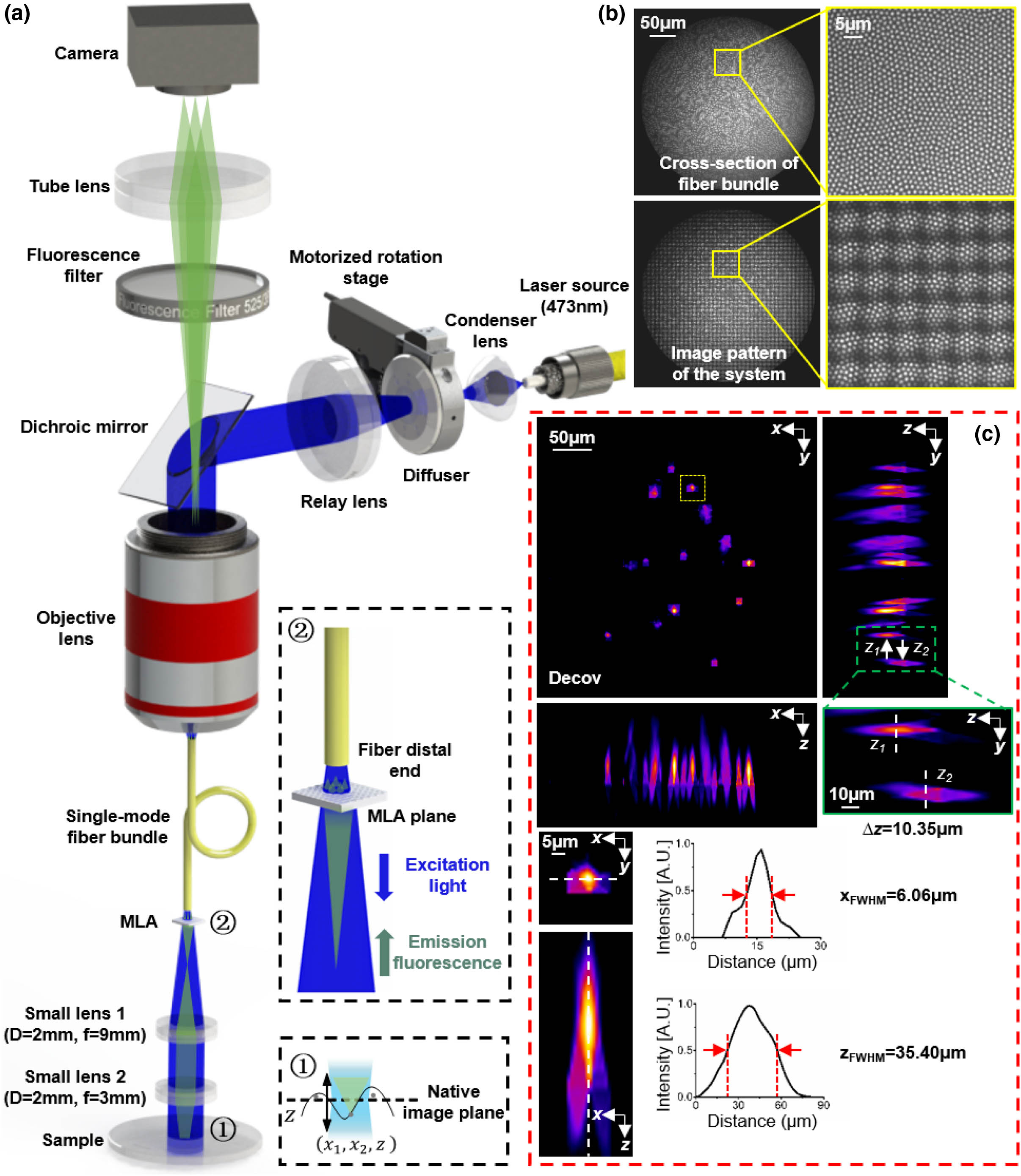
Figure 1.Principle of LFME. (a) Light-field micro-endoscopy (LFME) imaging scheme. The compact LFME system mainly consists of a small-size imaging lens pair, a small-size micro-lens array (MLA), and a single-mode fiber bundle (SMFB). Zoom-in panel ① shows the relationship of a sample space point with the native image plane (NIP). Zoom-in panel ② shows the enlarged image of the excitation light passing through the fiber distal end to the MLA plane and the emission light passing back. Note that on the illumination side, we use a rotating diffuser to weaken the spatial coherence of the laser source and reduce the speckle noise. (b) Cross-section image and its enlarged view of the SMFB (top), and the real image pattern and its enlarged view of the entire LFME system (bottom). (c) Experimental performance test by imaging randomly distributed fluorescent beads. The lateral and axial maximum intensity projections (MIPs) of beads are shown, after performing the Richardson–Lucy (RL) deconvolution. The resolved FWHM is 6.06 μm in the
The combination of SMFB, small lens pair, and MLA works as the imaging probe for direct tissue detection. The whole probe has a 2 mm diameter and is about 50 cm long. To realize three times magnification imaging, the imaging lens pair forms a 4f system, consisting of a small lens with a focal length
The optical design of our system has some particularities compared with the traditional epi-fluorescence light-field microscopy. We list some key points here. (1) Speckle noises. The fiber cores of SMFB in use will introduce moderate speckles when the coherent laser source is applied for epi-illumination, which will affect the imaging quality to a certain extent. Therefore, after the laser source, we place a continuously rotating diffuser (DG10-1500-MD, Thorlabs) to reduce the light coherence, driven by a motorized rotation stage (PRM1Z8, Thorlabs). For higher light efficiency, we use a condenser lens (ACL25416U-A, Thorlabs) for converging the light, and the diffuser is placed at the focal plane of the condenser. A relay lens is then applied for collimating the light. The comparison of different imaging performance with and without this rotating diffuser will be described in Section 3.D. (2) Sampling (pixelization) effect by SMFB. If we directly apply the SMFB for imaging, the spatial resolution will have an upper limit of
B. LFME Principle
In this work, we add a small lens pair and a small-size MLA in front of SMFB to realize the LFME system [Fig. 1(a)]. As mentioned above, by applying a resample step, the light-field image captured by our LFME is similar to the traditional light-field image. The effectiveness of the resample step is demonstrated experimentally in Appendix B. We thus can use the traditional Richardson–Lucy (RL) deconvolution [27,28] for reconstruction or apply the improved schemes [29,30] for artifact suppression. We just need to fine-tune the parameters in the algorithms according to the characteristics of the current data. Therefore, the image formation of LFME is the same as for traditional light-field microscopy [27,28].
1. Imaging Model and RL Deconvolution in LFME
We denote the sample space coordinate as
Here
For image reconstruction, we first resample and realign the captured light-field image into
2. Dictionary Learning Procedure in LFME
We further introduce the dictionary learning procedure [29] into our proposed LFME for artifact-suppressed and contrast-enhanced reconstruction performance. As the flow chart shows in Fig. 2, the dictionary learning reconstruction process can be decomposed into three parts: calibration, reconstruction through a few runs of RL iterations, and dictionary patching. In the calibration step, the captured light-field image is still resampled and realigned into
![]()
Figure 2.Dictionary learning procedure of LFME.
3. RESULTS
A. Fluorescence Imaging with LFME
Fluorescence endoscopy is a promising and useful technique in observing tissues, organs, and viscera of model animals or humans [1–3,14,31,32]. One application is the detection of gastrointestinal diseases, such as autofluorescence imaging of the gastrointestinal tract [1], detection of dysplasia in ulcerative colitis [2], and detection of non-visible malignant or premalignant lesions [3]. The proposed LFME is a good alternative for providing 3D fluorescence imaging.
We exhibit the fluorescence imaging of a human skin tissue section by using the LFME system in Fig. 3. The raw image in Fig. 3(a) is the light-field measurement, captured by assembling both the imaging lens pair and MLA. The raw image in Fig. 3(b) is captured only by using the imaging lens pair and serves as a reference image, which theoretically has higher spatial resolution since no MLA is applied. However, its real imaging performance is heavily contaminated by the pixelation effect of fiber cores, which is a common problem in wide-field imaging systems using SMFB. It also has a low imaging contrast with significant background fluorescence. Benefiting from our optical design of the LFME system, after performing the resample step and RL deconvolution [27,28] to the light-field measurement, our method can resolve fine details [Fig. 3(c)] similar to that of Fig. 3(b). The recovered image is with higher quality and cleaner background, although the raw light-field measurement in Fig. 3(a) is also heavily affected by the pixelation effect and noisy background. Moreover, by applying the dictionary learning method after deconvolution [29], we can further suppress artifacts and increase the image contrast, resolving more detailed structures of the skin tissue [Fig. 3(d)]. The intensity curves in Fig. 3(f), indicated by the red and blue lines in Figs. 3(c) and 3(d), can better present the artifact suppression ability of the dictionary learning method.
![]()
Figure 3.Fluorescence imaging with LFME. (a) Raw fluorescence light-field image of the human skin tissue. (b) Raw fluorescence image captured without MLA as a reference. Both images have heavy pixelation and large background fluorescence. Reconstructed fluorescence imaging in a certain slice using (c) RL deconvolution (Decov) and (d) dictionary learning after deconvolution (Decov+Dict), respectively. Benefiting from the optical design and reconstruction process of LFME, our method can resolve detailed structures of the skin tissue from (a) with a clean background. As shown in the enlarged drawings marked by the yellow box and the intensity curve in (f), dictionary learning can suppress artifacts and increase the contrast of reconstruction. (e1) is the central view image of a USAF-1951 resolution chart, while (e2) and (e3) are the reconstruction results using RL deconvolution and dictionary learning after deconvolution, respectively. Intensity curves shown in (g) correspond to the red, orange, and blue lines in (e1), (e2), and (e3), respectively.
We also image a USAF-1951 resolution chart attached with a fluorescent board as the object for lateral resolution evaluation of our LFME system, since we could not find a proper fluorescent chart for the performance test. As shown in Fig. 3(e3), by applying dictionary learning after deconvolution, group 7 line 1 of the resolution chart can be clearly distinguished, corresponding to at least 3.91 μm lateral resolution. The resolved lateral resolution can also be verified by the blue line of the intensity curve shown in Fig. 3(g).
B. Imaging Performance Analysis of LFME
In this section, we use several experiments to qualitatively and quantitatively analyze the imaging performance of the proposed LFME, such as (1) lateral resolution and FoV, (2) DoF and working distance, and (3) 3D imaging ability and axial resolution. To better demonstrate the improvement of our method, we also directly apply the SMFB (without assembling the lens pair and MLA) to fluorescence imaging as a reference for imaging performance comparisons.
1. Lateral Resolution and FoV
As shown in Figs. 3(e3) and 3(f), our method can obtain
![]()
Figure 4.Lateral resolution analysis for LFME. (a) Simulated LFME measurements of a point source in different axial positions. (b) Deconvolved images of a point source in different axial positions. (c) Experimentally characterized lateral resolution by imaging the resolution chart. (d) The simulated modulation transfer function (MTF) varies across different depths.
![]()
Figure 5.Fluorescence imaging by directly applying SMFB. From (a1)–(a8), the resolution chart is successively placed 0–25 μm away from the distal end of SMFB. (b1)–(b8) show corresponding enlarged drawings.
2. DoF and Working Distance
As a light-field endoscope, our method can largely extend the imaging DoF. The theoretical optimal DoF of our method can be calculated by simulations, which is determined by MTFs with the largest bandwidth. As shown in Fig. 4(d), the theoretical optimal DoF has an extremely large range. However, as mentioned before, the real optimal imaging depth range (maintaining
3. 3D Imaging Ability and Axial Resolution
Here we test the 3D imaging ability of our LFME system by imaging some randomly distributed fluorescence beads. We calculate and plot the lateral and axial MIPs of beads in Fig. 1(c). Specifically, we can identify different
C. 3D Imaging of Biological Samples with LFME
Previously, we have demonstrated the 3D imaging ability by imaging some fluorescence beads. In this section, we further exhibit the 3D imaging of some biological samples in Fig. 6. We compare different reconstruction results using both RL deconvolution and the dictionary learning method. As shown in Figs. 6(a1) and 6(a2), we present the recovered lateral (
![]()
Figure 6.3D imaging of biological samples with LFME. (a1) Recovered lateral (
D. Effectiveness of Rotating Diffuser in LFME
For practical use, we adopt the epi-illumination mode for fluorescence endoscopic imaging in this work, which means the illumination light will pass through the SMFB before being projected on the sample. Due to the coherence of the laser source in use, cross-talk among different fiber cores will introduce undesirable interference and speckles into the illumination, resulting in the degradation of the imaging quality. Therefore, after the laser source, we use a continuously rotating diffuser, driven by a motorized rotation stage, to weaken the spatial coherence of the laser source, as the optical system shown in Fig. 1(a).
In this section, we use experimental imaging of the fluorescent plate, HeLa cells, and skin tissue to demonstrate the effectiveness of the rotating diffuser in LFME, and the results are shown in Fig. 7. It should be noted that the images in the former three columns of Fig. 7 directly use the lens pair for acquisition without using the MLA, while the images in the last column use both the lens pair and the MLA (i.e., the input raw light-field measurement). As shown in the first column of Fig. 7, without the diffuser, the images are contaminated by undesirable interference patterns and speckles. By applying a diffuser, the interference pattern is suppressed, but the speckles still exist, as shown in the second column of Fig. 7. By rotating the diffuser continuously, we can eliminate the speckles of images (in the third column of Fig. 7), since the spatial coherence of the laser source is weakened. Finally, by further assembling the MLA, the raw light-field measurement can be captured (in the last column of Fig. 7), from which we can get reconstructed images with high resolution and clean backgrounds [Figs. 7(b5) and 7(c5)].
![]()
Figure 7.Effectiveness of rotating diffuser in LFME. We show experimentally captured images of the fluorescent plate, HeLa cells, and skin tissue to demonstrate the effectiveness of rotating diffuser in LFME. The former three columns directly use the lens pair for acquisition without using the MLA. The first column indicates imaging without the diffuser, which has undesirable interference patterns (labeled by yellow arrows) and speckles. The second column indicates imaging by applying a diffuser, where the interference pattern is suppressed, but the speckles still exist. The third column indicates imaging by rotating the diffuser continuously to weaken the spatial coherence of the laser source, where the speckles are eliminated at this time. The last column uses both the lens pair and MLA with diffuser rotation for image acquisition, which indicates the input raw light-field measurement. (b5) and (c5) are the reconstructed images with high resolution and clean backgrounds from the raw light-field measurements.
As we have mentioned before, in this work, we put the MLA between the SMFB and the imaging lens pair to avoid the information loss caused by the spatial sampling of fiber cores, which means the excitation light will also transmit through the MLA [Fig. 1(a)]. Fortunately, by comparing the captured light-field measurements (the last column of Fig. 7) with the reference images (the third column of Fig. 7), we can find that transmitting through the MLA will hardly change the light intensity distribution on the sample. Since the spatially sampling patterns introduced by fiber cores can be eliminated by the above-mentioned resample step, the light-field deconvolution process can be performed successfully, as the final imaging performance is shown in Figs. 7(b5) and 7(c5).
4. DISCUSSION
In summary, we develop LFME, a light-field micro-endoscopy technique, that can acquire 3D information in a compact epi-fluorescence endoscopic system with relatively low invasion (2-mm imaging probe). We utilize a dictionary learning method for deconvolution to mitigate the reconstruction artifacts and increase the imaging contrast. We demonstrate the snapshot 3D imaging performance of LFME through experiments of beads, HeLa cells, and a human skin section, preserving better than 6.20 μm lateral resolution within
Since the volume acquisition rate of LFME is only limited by the camera framerate, further improvement may rely on developing real integrated equipment of LFME rather than the proof-of-concept system in this paper for high-speed 3D
Acknowledgment
Acknowledgment. The authors thank Dr. Xuemei Hu for discussions.
APPENDIX A: OPTICAL PARAMETER SETTING
In this section, we present the details of the optical parameter setting.
APPENDIX B: REMOVAL OF PIXELIZATION EFFECT
In this section, we compare the raw light-field images before and after the resample step to illustrate the removal of cores. As shown in Fig.
![]()
Figure 8.Comparison of light-field measurements before (left) and after (right) the resample step.
APPENDIX C: NECESSITY OF ROTATING THE DIFFUSER
In this section, we compare the different reconstruction performance of light-field images captured with and without rotating the diffuser. The image of HeLa cells captured with diffuser rotation and no MLA is shown in Fig.
![]()
Figure 9.Comparison of light-field deconvolution with and without rotating the diffuser.
APPENDIX D: SIMILARITY OF PSFS BEFORE AND AFTER FIBER BUNDLE
In this section, we compare PSFs before and after light transmitting through the fiber bundle by imaging fluorescent beads. As shown in Fig.
![]()
Figure 10.Comparison of system’s PSFs before and after the fiber bundle by imaging fluorescent beads.
APPENDIX E: LATERAL RESOLUTION IN A LARGER DoF
In this section, we test the lateral resolution of our system in a larger DoF. As mentioned, the optimal DoF of this work is defined as the optimal axial range that can preserve better than 6.20 μm lateral resolution. Outside this optimal range, our method can still work but with a certain degree of resolution loss. As shown in Fig.
![]()
Figure 11.Lateral resolution testing in a larger DoF.
APPENDIX F: HARDWARE AND SOFTWARE CONFIGURATION
In this work, we process the data using MATLAB software in a 64 bit computer with Intel Core i7-8700 CPU at 3.20 GHz and 32 GB RAM. The generation of the simulated PSF matrix (based on system parameters) with 43 axial layers takes about 255 s, and the process only needs to be conducted once in advance. The RL deconvolution (five times) of the resampled light-field image with
APPENDIX G: SAMPLE PREPARATION
In this section, we present the details of sample preparations.
References
[1] H. Tajiri. Autofluorescence endoscopy for the gastrointestinal tract. Proc. Jpn. Acad. B, 83, 248-255(2007).
[2] H. Messmann, E. Endlicher, G. Freunek, P. Rümmele, J. Schoelmerich, R. Knüchel. Fluorescence endoscopy for the detection of low and high grade dysplasia in ulcerative colitis using systemic or local 5-aminolaevulinic acid sensitisation. Gut, 52, 1003-1007(2003).
[3] H. Messmann, E. Endlicher, C. Gelbmann, J. Schoelmerich. Fluorescence endoscopy and photodynamic therapy. Dig. Liver Dis., 34, 754-761(2002).
[4] J. J. Tjalma, M. Koller, M. D. Linssen, E. Hartmans, S. De Jongh, A. Jorritsma-Smit, A. Karrenbeld, E. G. de Vries, J. H. Kleibeuker, J. P. Pennings, K. Havenga, P. H. Hemmer, G. A. Hospers, B. van Etten, V. Ntziachristos, G. M. van Dam, D. J. Robinson, W. B. Nagengast. Quantitative fluorescence endoscopy: an innovative endoscopy approach to evaluate neoadjuvant treatment response in locally advanced rectal cancer. Gut, 69, 406-410(2020).
[5] A. D. Jacob, A. I. Ramsaran, A. J. Mocle, L. M. Tran, C. Yan, P. W. Frankland, S. A. Josselyn. A compact head-mounted endoscope for
[6] Z. Qin, C. Chen, S. He, Y. Wang, K. F. Tam, N. Y. Ip, J. Y. Qu. Adaptive optics two-photon endomicroscopy enables deep-brain imaging at synaptic resolution over large volumes. Sci. Adv., 6, eabc6521(2020).
[7] W. Zong, R. Wu, M. Li, Y. Hu, Y. Li, J. Li, H. Rong, H. Wu, Y. Xu, Y. Lu, H. Jia, M. Fan, Z. Zhou, Y. Zhang, A. Wang, L. Chen, H. Cheng. Fast high-resolution miniature two-photon microscopy for brain imaging in freely behaving mice. Nat. Methods, 14, 713-719(2017).
[8] S. A. Vasquez-Lopez, R. Turcotte, V. Koren, M. Plöschner, Z. Padamsey, M. J. Booth, T. Čižmár, N. J. Emptage. Subcellular spatial resolution achieved for deep-brain imaging
[9] A. Hassanfiroozi, Y.-P. Huang, B. Javidi, H.-P. D. Shieh. Hexagonal liquid crystal lens array for 3D endoscopy. Opt. Express, 23, 971-981(2015).
[10] Y. Zhang, M. L. Akins, K. Murari, J. Xi, M.-J. Li, K. Luby-Phelps, M. Mahendroo, X. Li. A compact fiber-optic SHG scanning endomicroscope and its application to visualize cervical remodeling during pregnancy. Proc. Natl. Acad. Sci. USA, 109, 12878-12883(2012).
[11] Z. Qiu, W. Piyawattanametha. MEMS actuators for optical microendoscopy. Micromachines, 10, 85(2019).
[12] B. A. Flusberg, A. Nimmerjahn, E. D. Cocker, E. A. Mukamel, R. P. Barretto, T. H. Ko, L. D. Burns, J. C. Jung, M. J. Schnitzer. High-speed, miniaturized fluorescence microscopy in freely moving mice. Nat. Methods, 5, 935-938(2008).
[13] E. R. Andresen, S. Sivankutty, V. Tsvirkun, G. Bouwmans, H. Rigneault. Ultrathin endoscopes based on multicore fibers and adaptive optics: a status review and perspectives. J. Biomed. Opt., 21, 121506(2016).
[14] B. A. Flusberg, E. D. Cocker, W. Piyawattanametha, J. C. Jung, E. L. Cheung, M. J. Schnitzer. Fiber-optic fluorescence imaging. Nat. Methods, 2, 941-950(2005).
[15] C. Xia, M. A. Eftekhar, R. A. Correa, J. E. Antonio-Lopez, A. Schülzgen, D. Christodoulides, G. Li. Supermodes in coupled multi-core waveguide structures. IEEE J. Sel. Top. Quantum Electron., 22, 196-207(2015).
[16] V. Szabo, C. Ventalon, V. De Sars, J. Bradley, V. Emiliani. Spatially selective holographic photoactivation and functional fluorescence imaging in freely behaving mice with a fiberscope. Neuron, 84, 1157-1169(2014).
[17] R. Florentin, V. Kermene, J. Benoist, A. Desfarges-Berthelemot, D. Pagnoux, A. Barthélémy, J.-P. Huignard. Shaping the light amplified in a multimode fiber. Light Sci. Appl., 6, e16208(2017).
[18] N. Badt, O. Katz. Label-free video-rate micro-endoscopy through flexible fibers via Fiber Bundle Distal Holography (FiDHo)(2021).
[19] J. Shin, D. N. Tran, J. R. Stroud, S. Chin, T. D. Tran, M. A. Foster. A minimally invasive lens-free computational microendoscope. Sci. Adv., 5, eaaw5595(2019).
[20] A. Orth, M. Ploschner, E. Wilson, I. Maksymov, B. Gibson. Optical fiber bundles: ultra-slim light field imaging probes. Sci. Adv., 5, eaav1555(2019).
[21] A. Orth, M. Ploschner, I. S. Maksymov, B. C. Gibson. Extended depth of field imaging through multicore optical fibers. Opt. Express, 26, 6407-6419(2018).
[22] C. Guo, T. Urner, S. Jia. 3D light-field endoscopic imaging using a GRIN lens array. Appl. Phys. Lett., 116, 101105(2020).
[23] T. M. Urner, A. Inman, B. Lapid, S. Jia. Three-dimensional light-field microendoscopy with a GRIN lens array. Biomed. Opt. Express, 13, 590-607(2022).
[24] J. Liu, D. Claus, T. Xu, T. Kessner, A. Herkommer, W. Osten. Light field endoscopy and its parametric description. Opt. Lett., 42, 1804-1807(2017).
[25] Y. Xue, I. G. Davison, D. A. Boas, L. Tian. Single-shot 3D wide-field fluorescence imaging with a computational miniature mesoscope. Sci. Adv., 6, eabb7508(2020).
[26] K. Yanny, N. Antipa, W. Liberti, S. Dehaeck, K. Monakhova, F. L. Liu, K. Shen, R. Ng, L. Waller. Miniscope3D: optimized single-shot miniature 3D fluorescence microscopy. Light Sci. Appl., 9, 171(2020).
[27] M. Broxton, L. Grosenick, S. Yang, N. Cohen, A. Andalman, K. Deisseroth, M. Levoy. Wave optics theory and 3-D deconvolution for the light field microscope. Opt. Express, 21, 25418-25439(2013).
[28] R. Prevedel, Y.-G. Yoon, M. Hoffmann, N. Pak, G. Wetzstein, S. Kato, T. Schrödel, R. Raskar, M. Zimmer, E. S. Boyden, A. Vaziri. Simultaneous whole-animal 3D imaging of neuronal activity using light-field microscopy. Nat. Methods, 11, 727-730(2014).
[29] Y. Zhang, B. Xiong, Y. Zhang, Z. Lu, J. Wu, Q. Dai. DiLFM: an artifact-suppressed and noise-robust light-field microscopy through dictionary learning. Light Sci. Appl., 10, 152(2021).
[30] Z. Lu, J. Wu, H. Qiao, Y. Zhou, T. Yan, Z. Zhou, X. Zhang, J. Fan, Q. Dai. Phase-space deconvolution for light field microscopy. Opt. Express, 27, 18131-18145(2019).
[31] M. Gu, H. Bao, H. Kang. Fibre-optical microendoscopy. J. Microsc., 254, 13-18(2014).
[32] R. P. Barretto, T. H. Ko, J. C. Jung, T. J. Wang, G. Capps, A. C. Waters, Y. Ziv, A. Attardo, L. Recht, M. J. Schnitzer. Time-lapse imaging of disease progression in deep brain areas using fluorescence microendoscopy. Nat. Med., 17, 223-228(2011).
[33] H. Pahlevaninezhad, M. Khorasaninejad, Y.-W. Huang, Z. Shi, L. P. Hariri, D. C. Adams, V. Ding, A. Zhu, C.-W. Qiu, F. Capasso, M. J. Suter. Nano-optic endoscope for high-resolution optical coherence tomography
[34] M. Chen, Z. F. Phillips, L. Waller. Quantitative differential phase contrast (DPC) microscopy with computational aberration correction. Opt. Express, 26, 32888-32899(2018).
[35] J. Chung, G. W. Martinez, K. C. Lencioni, S. R. Sadda, C. Yang. Computational aberration compensation by coded-aperture-based correction of aberration obtained from optical Fourier coding and blur estimation. Optica, 6, 647-661(2019).
[36] S. Abrahamsson, J. Chen, B. Hajj, S. Stallinga, A. Y. Katsov, J. Wisniewski, G. Mizuguchi, P. Soule, F. Mueller, C. D. Darzacq, X. Darzacq, C. Wu, C. I. Bargmann, D. A. Agard, M. Dahan, M. G. L. Gustafsson. Fast multicolor 3D imaging using aberration-corrected multifocus microscopy. Nat. Methods, 10, 60-63(2013).


Set citation alerts for the article
Please enter your email address

© Copyright 2018-2021 | Chinese Laser Press. All Rights Reserved 沪ICP备15018463号-20