High-Q, low-mode-volume microsphere-integrated Fabry–Perot cavity for optofluidic lasing applications

Xiaoqin Wu; Yipei Wang; Qiushu Chen; Yu-Cheng Chen; Xuzhou Li; Limin Tong; Xudong Fan

doi:10.1364/PRJ.7.000050

Journals >Photonics Research >Volume 7 >Issue 1 >Page 50 > Article

Photonics Research
Vol. 7, Issue 1, 50 (2019)

High-Q, low-mode-volume microsphere-integrated Fabry–Perot cavity for optofluidic lasing applications

Xiaoqin Wu^1、2, Yipei Wang³, Qiushu Chen¹, Yu-Cheng Chen¹, Xuzhou Li¹, Limin Tong², and Xudong Fan^1、*

Author Affiliations

¹Department of Biomedical Engineering, University of Michigan, Ann Arbor, Michigan 48109, USA

²State Key Laboratory of Modern Optical Instrumentation, College of Optical Science and Engineering, Zhejiang University, Hangzhou 310027, China

³Department of Electrical & Computer Engineering, University of Michigan, Ann Arbor, Michigan 48109, USA

show less

DOI: 10.1364/PRJ.7.000050 Cite this Article Set citation alerts

Xiaoqin Wu, Yipei Wang, Qiushu Chen, Yu-Cheng Chen, Xuzhou Li, Limin Tong, Xudong Fan. High-Q, low-mode-volume microsphere-integrated Fabry–Perot cavity for optofluidic lasing applications[J]. Photonics Research, 2019, 7(1): 50 Copy Citation Text

EndNote(RIS)

BibTex

Plain Text

show less

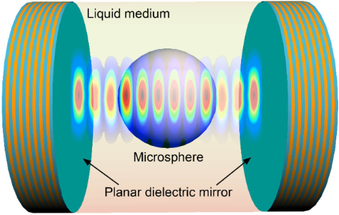
Fig. 1. Schematic of an MIFP cavity, in which an MS is inserted in an FP cavity filled with liquid.

Download full size | View in the Article

(a) and (b), (d)–(g) Schematic and representative electrical field distribution of the fundamental resonant mode of (a) and (b) MIFP, (d) and (e) finite PPFP, and (f) and (g) WGM cavities, respectively. d is the diameter of the MSs and also the diameter of the circular mirrors. L is the mirror spacing. For the MIFP cavity, the MS is assumed in the center of the two mirrors. In (b), (e), and (g), the parameters are d=3 μm, L=3.06 μm, and na=1.33. The symmetrical axis is set in the 2D-axisymmetric model, indicating the geometry on the right side is assumed to rotate around the axis, rendering a quasi-3D model. PMLs are boundaries where the calculation is terminated. Integration line R in (b) is plotted across the vertical center of the freestanding wave node closest to the bottom mirror and is used to calculate the effective mode radius. (c) Reflectance spectra of 7-, 11-, and 15-dielectric-layer mirrors across a wavelength range of 400 to 800 nm. (h) Q-factor of MIFP, finite PPFP, and WGM cavities as a function of d. There are two variables (d and L) for the MIFP cavity and the PPFP cavity. For a given d, L is chosen to be as close to d as possible and with maximum calculated Q-factor for the MIFP cavity in a range of L from d+0.02 to d+0.28 μm, since the Q-factor oscillates over L with a period of about 0.28 μm.

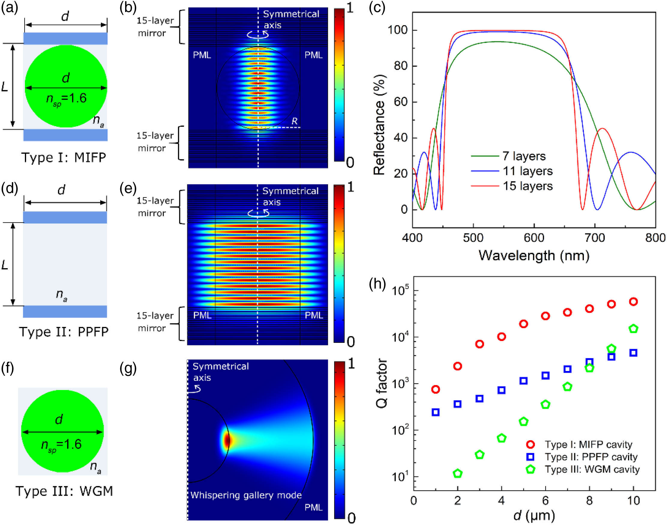
Fig. 2. (a) and (b), (d)–(g) Schematic and representative electrical field distribution of the fundamental resonant mode of (a) and (b) MIFP, (d) and (e) finite PPFP, and (f) and (g) WGM cavities, respectively. d is the diameter of the MSs and also the diameter of the circular mirrors. L is the mirror spacing. For the MIFP cavity, the MS is assumed in the center of the two mirrors. In (b), (e), and (g), the parameters are d=3 μm, L=3.06 μm, and na=1.33. The symmetrical axis is set in the 2D-axisymmetric model, indicating the geometry on the right side is assumed to rotate around the axis, rendering a quasi-3D model. PMLs are boundaries where the calculation is terminated. Integration line R in (b) is plotted across the vertical center of the freestanding wave node closest to the bottom mirror and is used to calculate the effective mode radius. (c) Reflectance spectra of 7-, 11-, and 15-dielectric-layer mirrors across a wavelength range of 400 to 800 nm. (h) Q-factor of MIFP, finite PPFP, and WGM cavities as a function of d. There are two variables (d and L) for the MIFP cavity and the PPFP cavity. For a given d, L is chosen to be as close to d as possible and with maximum calculated Q-factor for the MIFP cavity in a range of L from d+0.02 to d+0.28 μm, since the Q-factor oscillates over L with a period of about 0.28 μm.

Download full size | View in the Article

Fig. 3. (a)–(d) Electrical field distribution of the (a) HE11, (b) TM01, (c) TE01, and (d) HE21 modes of an MIFP cavity with a 2-μm diameter MS placed in a 2.04-μm-long FP cavity (d=2 μm, L=2.04 μm, na=1.5). Upper and lower panels are the cross-sectional and vertical-sectional view, respectively. White arrows indicate the in-plane electrical field vector in the cross-sectional view. (e)–(g) Q-factor of the HE11, TM01, TE01, and HE21 modes as a function of surrounding medium RI na for three different MIFP structures: (e) 1-μm MS in 1.04-μm-long cavity (d=1 μm, L=1.04 μm), (f) 2-μm MS in 2.04-μm-long cavity (d=2 μm, L=2.04 μm), and (g) 4-μm MS in 4.06-μm-long cavity (d=4 μm, L=4.06 μm). The diameter of the mirrors is set to be 2 μm larger than that of the corresponding MS.

Download full size | View in the Article

Fig. 4. Electrical field distribution of the HE21 mode of the MIFP cavity in Fig. 3(e) (d=1 μm, L=1.04 μm) (a) before and (b) after the Q-factor drop as the surrounding medium RI na increases from (a) 1.5 to (b) 1.52. It can be seen that the mode confinement in (b) becomes quite weak with a large portion of the eletrical field leaking into the PML layer, leading to an extra spillover loss and a decreased Q-factor.

Download full size | View in the Article

Fig. 5. (a) Schematic of an MIFP cavity with the cavity length L larger than the MS diameter d. b0 is the distance from the MS center to the bottom mirror. (b) Electrical field amplitude distribution of the HE11 mode for MIFP cavities (d=4 μm, b0=2.03 μm) with cavity lengths L=6 μm and 8 μm under a surrounding medium RI of 1.33, 1.4, and 1.5, respectively. (c)–(e) Calculated Q-factor of HE11 mode for MIFP cavities (d=4 μm, b0=2.03 μm) as a function of cavity length L at (c) na=1.33, (d) na=1.4, and (e) na=1.5, respectively. In the observation window of 520–560 nm for the resonance wavelength, there are usually two modes with consecutive longitudinal mode numbers but different Q. For clarity, we divide them into two groups. The red circle line corresponds to even longitudinal mode numbers (m=2N), and the blue circle line corresponds to odd longitudinal mode numbers (m=2N+1). (f)–(h) Calculated Q-factor of the TM01, TE01, and HE21 modes for MIFP cavities (d=4 μm, b0=2.03 μm) as a function of cavity length L at (f) na=1.33, (g) na=1.4, and (h) na=1.5, respectively.

Download full size | View in the Article

Fig. 6. (a)–(c) Photonic nanojet formation by a 4-μm diameter polystyrene MS illuminated by a Guassian beam (radius=3 μm) with a surrounding medium RI of (a) na=1.33, (b) na=1.4, and (c) na=1.5. The point with the maximal electric field amplitude is chosen to be the focusing point. The focal length here is defined as the distance from the bottom of the MS to the focusing point. (d) Reflected light field distribution when the “nanojet” formed in (a) is incident on a mirror placed within the focusing length of the MS at na=1.33. Most of the light field is reflected back into the MS. (e) Reflected light field distribution when the “nanojet” formed in (a) is incident on a mirror placed beyond the focusing length of the MS at na=1.33. A large portion of the light field misses the MS. For a better understanding, the nanojet formation is simplified as a focusing lens in ray optics, as shown in insets of (d) and (e). Schematics show how light propagates when the mirror is placed within [inset of (d)] and outside [inset of (e)] the focusing plane.

Download full size | View in the Article

Fig. 7. (a)–(c) Calculated Q-factors of the HE11, TM01, TE01, and HE21 modes as a function of b0 [the distance from the MS center to the bottom mirror, illustrated in Fig. 5(a)] at (a) na=1.33, (b) na=1.4, and (c) na=1.5 for the MIFP cavity with fixed d=4 μm and L=6 μm. (d)–(f) Calculated Q-factors of the HE11, TM01, TE01, and HE21 modes as a function of b0 at (d) na=1.33, (e) na=1.4, and (f) na=1.5 for the MIFP cavity with fixed d=4 μm and L=10 μm. Insets in (d) and (e) show the HE11 mode profiles at b0=4.9 μm and 4.48 μm, respectively.

Download full size | View in the Article

Fig. 8. (a) Schematic of an MIFP cavity with the top mirror tilted by θ with respect to the bottom mirror. (b) Fundamental mode profile of an MIFP cavity (d=4 μm, L=6.18 μm, na=1.4, θ=2°). (c)–(e) Comparison of the Q-factor of the fundamental mode under different tilting angles (θ=0°, 1°, and 2°), and cavity length L is set to be 1, 1.5, and 2 times the MS diameter d at (c) na=1.33, (d) na=1.4, and (e) na=1.5.

Download full size | View in the Article

Fig. 9. (a) Lasing spectra for MIFP-based lasers constructed by inserting 4-μm (red line), 2-μm (blue line), and 1-μm (green line) diameter polystyrene MSs between the two mirrors. Insets show the images of the lasing modes. Scale bar, 2 μm. (b) Spectrally integrated laser output as a function of pump energy density for the 4-μm diameter MIFP (red) and 2-μm diameter MIFP (blue) cavity, respectively. (c) Spectrally integrated laser output as a function of pump energy density for the 1-μm diameter MIFP cavity.

Download full size | View in the Article

Fig. 10. (a) Lasing spectra under different pump intensity for MIFP-based lasers constructed by inserting a 4-μm diameter polystyrene MS (indicated by the dashed circle in the inset) into a 6-μm length FP cavity. The cavity spacing is controlled by using 6-μm diameter non-fluorescent MSs (indicated by the dashed circles in the inset). Scale bar, 4 μm. (b) Spectrally integrated laser output as a function of pump energy density for the MIFP-based laser in (a). Error bars are obtained by 3 measurements.

Download full size | View in the Article

$d$ (μm)	$L$ (μm)	$n_{a}$	$Q$ -factor	Finesse	$r_{m}$ (μm)	$V_{eff}$ ( ${μm}^{3}$ )
1	1.04	1.33	757.7	126.3	0.261	0.084
		1.4	1165.6	194.3	0.275	0.098
		1.5	3264.2	544	0.316	0.150
		1.56	12037	2006.2	0.422	0.334
2	2.04	1.33	2354.1	196.2	0.326	0.290
		1.4	3654.4	304.5	0.339	0.362
		1.5	8003.5	667.0	0.381	0.568
		1.58	26710	2225.8	0.556	1.366
4	4.06	1.33	3387.8	141.2	0.457	1.169
		1.4	19771	823.8	0.476	1.489
		1.5	20273	844.7	0.571	2.232
		1.58	59875	2494.8	0.853	5.144

Table 1. Q-Factor, Finesse, Mode Radius, and Mode Volume (HE11 Mode) of MIFP Cavity at a Wavelength around 540 nm^a

View in the Article

Dye concentration $N$	12 mmol/L ( $7.4 \times 10^{18} {cm}^{- 3}$ )
Pump wavelength $λ_{p}$ (nm)	479
Absorption cross section at $λ_{p}$ ( ${cm}^{2}$ )	$1.222 \times 10^{- 16}$
Refractive index of the microsphere $n_{sp}$	1.6
Pulse width $Δ t$ (ns)	5
MIFP cavity (µm)	$L = d = 4$	$L = d = 2$	$L = d = 1$
Lasing wavelength $λ_{L}$ (nm)	552	517	536
Absorption cross section at $λ_{L}$ ( ${cm}^{2}$ )	$2.308 \times 10^{- 18}$	$2.864 \times 10^{- 17}$	$8.449 \times 10^{- 18}$
Emission cross section at $λ_{L}$ ( ${cm}^{2}$ )	$6.788 \times 10^{- 17}$	$1.22 \times 10^{- 16}$	$8.509 \times 10^{- 17}$
Fluorescence distribution $E (λ_{L})$ (nm^-1)	$8 \times 10^{- 3}$	$1.88 \times 10^{- 2}$	$1.13 \times 10^{- 2}$
$Q_{abs}$ at $λ_{L}$	10,663	917	3000
A	0.0189	0.2344	0.0691
B	0.034	0.2348	0.0993
$8 π h c^{2} n^{2} Δ t / λ_{L}^{4} λ_{p} E (λ_{L})$ ( $μJ / {mm}^{2}$ )	53.9	29.82	42.94
$P_{th}$ ( $μJ / {mm}^{2}$ )	1.9	10	50
$Q_{0}$	13,100	2844	506