Applications of weakly-coupled few-mode fibers [Invited]

Huiyuan Liu; He Wen; Guifang Li

doi:10.3788/COL202018.040601

Abstract

Space-division multiplexing (SDM) has attracted significant attention in recent years because larger transmission capacity is enabled by more degrees of freedom (DOFs) in few-mode fibers (FMFs) compared with single-mode fibers (SMFs). To transmit independent information on spatial modes without or with minor digital signal processing (DSP), weakly-coupled FMFs are preferred in various applications. Several cases with different use of spatial DOFs in weakly-coupled FMFs are demonstrated in this work, including single-mode or mode-group-multiplexed transmission, and spatial DOFs combined with time or frequency DOF to improve the system performance.

Keywords

few-mode fibers fiber optics links and subsystems fibers multiplexing nonlinear optics radio frequency photonics

1. INTRODUCTION

As the transmission capacity worldwide continues to grow exponentially and single-mode fiber-optic communication systems approach their capacity limit^[1,2], space-division multiplexing (SDM) has attracted significant attention in recent years^[3,4]. With more spatial modes in few-mode fibers (FMFs) or multicore fibers (MCFs), SDM enables a larger transmission capacity^[5], improved signal transmission performance, or enhanced signal processing ability compared with single mode fibers (SMFs)^[6] due to more degrees of freedom (DOFs)^[3].

Spatial modes in FMFs are orthogonal to each other ideally, so they can deliver different signals in independent channels. However, in practical fibers, there are unavoidable defects due to a limited fabrication accuracy or surrounding environment change, such as index profile fluctuation, geometry deviation, and microbending, leading to cross talk between different modes^[7–9].

To recover independent information from mode cross talk, digital signal processing (DSP) with multiple-input-multiple-output (MIMO) is usually needed to retrieve both amplitude and phase information of the received optical signal with the help of mature coherent detection techniques^[10]. However, due to the modal dispersion of FMFs, equalizers with a long memory are required in DSP^[11], which increases the complexity and cost of the whole system. Even with optimized fiber index profiles, equalization schemes, and algorithms, some transmission systems still suffer from the cost and power consumption of DSP components, especially those short-reach systems such as datacenter transmission systems^[12].

Sign up for Chinese Optics Letters TOC. Get the latest issue of Chinese Optics Letters delivered right to you！Sign up now

Weakly-coupled FMFs offer a cost-effective solution to address the above issues, since there is no need of MIMO DSP at the receiver end^[13]. Recently, there have been many references of designing weakly coupled FMFs^[14–16] that verify their application in mode-division multiplexing (MDM) transmission. The weak coupling benefits not only MDM, but also many other applications due to the large number of DOFs. Here we demonstrate several cases of the use of DOFs in weakly-coupled FMFs for different applications. First, we introduce long-haul quasi-single-mode transmission using only one element of spatial DOFs (one mode) in the FMFs^[17,18]. Second, we talk about the use of multiple elements of spatial DOFs (multiple modes) to realize MIMO-less mode-group multiplexing (MGM)^[19]. Finally, we show upstream transmission in time-division multiplexed (TDM) passive optical network (PON), and wavelength-division multiplexed (WDM) microwave photonics as examples of using spatial DOFs to improve the performance of systems assisted with time and frequency DOF^[20,21].

2. CONSIDERATIONS OF WEAKLY-COUPLED FMFs

Weakly-coupled FMFs can increase the fiber capacity without DSP, since different modes can carry different information with negligible cross talk. To study how to make FMFs weakly coupled, the coupling between different modes is analyzed here.

In an ideal FMF, spatial modes are orthogonal to each other, so there is no cross talk between different spatial modes, which can be seen from the coupling coefficient $K_{k j}$ calculation^[22] $K_{k j} = \frac{ω}{4} \iint_{\infty} d x d y Δ ε (x, y) {\vec{e}}_{k} (x, y) {\vec{e}}_{j}^{*} (x, y),$ (1)where $ω$ is the angular frequency, ${\vec{e}}_{k}$ , ${\vec{e}}_{j}$ are the transverse components of mode fields labeled $k$ , $j$ , and $Δ ε$ is the dielectric perturbation. If there is no or uniform dielectric perturbation, the coupling coefficient is zero. It is the foundation of transmitting different signals in different modes as distinct channels in the FMFs. However, those modes are easily coupled to each other in practical FMFs and non-ideal environments when the dielectric perturbation is not uniform over the cross section of fiber, which affects the system performance of FMFs^[9,23,24]. The coupling efficiency between modes is also affected by the phase-matching condition related to the effective index difference between modes, as shown in the coupled-mode equations of two modes, $\frac{d A_{1}}{d z} = i K_{11} A_{1} + i K_{12} A_{2} \exp [i (β_{2} - β_{1}) z], \frac{d A_{2}}{d z} = i K_{22} A_{2} + i K_{21} A_{1} \exp [i (β_{1} - β_{2}) z],$ (2)where $A_{1}$ , $A_{2}$ are the amplitudes for two modes, $β_{1}$ , $β_{2}$ are propagation constants of two modes, and coupling efficiencies $K_{12}$ , $K_{21}$ change with $Δ ε$ . From the coupled-mode equations, the coupling coefficients, which vary along the fiber, need to match the phase terms $\exp [\pm i (β_{2} - β_{1}) z]$ to produce a sufficient amplitude change, so the dielectric perturbation or the refractive index perturbation that meets the phase-match condition brings effective mode cross talk. Since the dielectric perturbation as a function of longitudinal spatial frequencies has dominant components at low frequencies, increasing the propagation constant difference or effective index difference between modes can reduce the mode cross talk significantly^[25,26]. When the effective index difference between adjacent modes is larger than $1 \times 10^{- 3}$ ^[15], the FMF can be regarded as being weakly coupled. For practical employment, the required effective index difference can be different for various system lengths or winding tensions^[23]. $1.7 \times 10^{- 3}$ is a good practical value as the target^[16,23].

To achieve that and ensure the same number of modes is supported in the fiber, both a large index contrast between the core and cladding and a small core diameter are needed^[27]. However, a small core diameter will reduce the effective areas of modes, which would increase nonlinearities in FMFs^[28], so here we study the trade-off between the large mode effective area and the large effective index difference between neighboring modes by theoretical analysis and numerical simulation.

Usually, effective areas of higher-order modes are larger than that of the fundamental mode, since they are less confined by the core^[29]. Nonlinearity is more concerned when the optical power is large in long-haul systems, where quasi-single-mode (QSM) transmission plays an important role. QSM usually transmits the fundamental mode, since it is easily launched and compatible with other single-mode components in the system^[18]. So the effective area of the fundamental mode is calculated here. In QSM transmission, the index difference between the fundamental mode and the first higher-order mode is a very important evaluator of the mode cross talk. For other applications with graded-index (GRIN) FMFs, there are almost equal index differences between neighboring mode groups^[30], so the effective index difference between the first two modes is computed here.

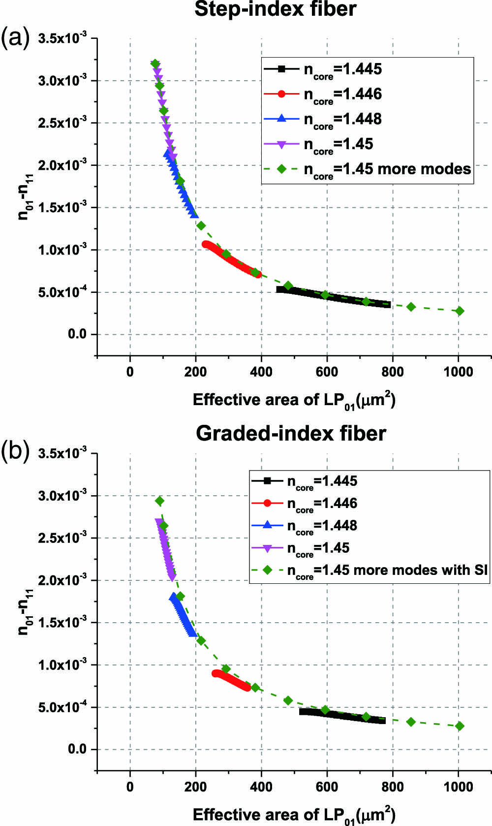
Figure 1 shows the effective index difference between first two modes as a function of the effective area of the fundamental mode in the two-mode step-index (SI) or GRIN fibers. For different core indices, the core radius is varying in a range to ensure that only two modes survive. The result of SI fiber with a fixed core index of 1.45 and a large range of core radii is plotted as the reference curve. Other curves are all overlapped with the reference curve, indicating that the multiplication of the effective index difference and the effective area is a constant, no matter how the index profile is varying. Figure 1(b) shows that the constant value for GRIN fiber is very close to and a little smaller than that for SI fiber.

Figure 1.Effective index difference between the first two modes, as a function of the effective area of the fundamental mode, with varying core radius for each core index, in (a) two-mode step-index fiber and (b) two-mode graded-index fiber. Step-index fiber with a 1.45 core index and a large range of core radius is plotted as the reference curve.

The multiplication of effective index difference and effective area seems to be a constant value for different fiber index profiles, which can be verified analytically for GRIN fibers. The Helmholtz equation for electrical field $E$ in a GRIN fiber can be written as $\nabla^{2} E + n^{2} k_{0}^{2} E = (\frac{\partial^{2}}{\partial x^{2}} + \frac{\partial^{2}}{\partial y^{2}}) E + (n^{2} k_{0}^{2} - β^{2}) E = 0,$ (3)where $n$ is the refractive index represented as $n^{2} = n_{1}^{2} - 2 n_{1}^{2} Δ {(r / a)}^{2}$ , $Δ = n_{1}^{2} - n_{2}^{2} / 2 n_{1}^{2}$ , $a$ is the core radius, n₁ and n₂ are refractive indices of core and cladding, $k_{0}$ is the free-space wave number, and $β$ is the propagation constant. The equation can be also written as^[31] $- (\frac{\partial^{2}}{\partial x^{2}} + \frac{\partial^{2}}{\partial y^{2}}) E + \frac{2 k_{1}^{2} Δ}{a^{2}} (x^{2} + y^{2}) E = (k_{1}^{2} - β^{2}) E,$ (4)where $k_{1} = n_{1}^{2} k_{0}^{2}$ . The solutions can be found as^[32] $k_{1}^{2} - β^{2} = 2 \sqrt{\frac{2 k_{1}^{2} Δ}{a^{2}}} (m_{x} + m_{y} + 1),$ (5) $β = \sqrt{k_{1}^{2} - k_{1} \frac{2 \sqrt{2 Δ}}{a} (m_{x} + m_{y} + 1)} \approx k_{1} - \frac{\sqrt{2 Δ}}{a} (m_{x} + m_{y} + 1) .$ (6)

From Eq. (6) the effective index difference between two neighboring modes is $Δ n = \frac{\sqrt{2 Δ}}{a k_{0}} .$ (7)

The fundamental solution of the electrical field can be approximated as the Gaussian function $E_{0} = A e^{- \frac{x^{2} + y^{2}}{2 σ^{2}}}$ , where $σ$ is the standard deviation of the Gaussian function as $σ^{2} = \frac{a}{k_{1} \sqrt{2 Δ}}$ ^[32,33]. The integral of a Gaussian function gives $\iint A e^{- \frac{x^{2} + y^{2}}{2 σ^{2}}} d x d y = 2 π A σ^{2},$ (8)and the effective area of ${LP}_{01}$ is calculated as $A_{eff} = \frac{{(\iint {| E |}^{2} d x d y)}^{2}}{\iint {| E |}^{4} d x d y} = 2 π σ^{2} = 2 π \frac{a}{k_{1} \sqrt{2 Δ}} .$ (9)

The multiplication of the effective area and index difference thus leads to the relation below: $A_{eff} Δ n = 2 π \frac{a}{k_{1} \sqrt{2 Δ}} \frac{\sqrt{2 Δ}}{a k_{0}} = \frac{λ_{0}^{2}}{2 π n_{1}} .$ (10)

It is a constant at a fixed core index and wavelength. When the constant is divided by the wavelength, the formula is only related to the core index in the following form: $\frac{A_{eff} Δ n}{λ_{0}^{2}} = \frac{1}{2 π n_{1}} .$ (11)

The value would be 0.1098 for a 1.45 core index. The fitting curve is plotted in Fig. 2(a), showing a fitting coefficient of 0.1097, which is almost the same as the analytical result.

Figure 2.(a) Effective index difference vs. effective area curve fitting for graded-index fiber. (b) The multiplication constant as a function of wavelength for SI or GRIN fibers with two or ten modes.

To verify that the formula $\frac{Δ n A_{eff}}{λ_{0}^{2}}$ is constant at different wavelengths, the numerical simulation results as functions of wavelength for SI or GRIN fibers with two or ten modes are plotted in Fig. 2(b). The curves for two-mode fibers show that the simulated value decreases slowly as the wavelength increases because it is closer to the cutoff condition at a longer wavelength. Far away from the cutoff condition, the curves for SI or GRIN fibers with ten modes demonstrate nearly constant values at different wavelengths.

The previous simulation shows that the multiplication of the effective index difference and the effective area of the fundamental mode is always a constant for common SI and GRIN FMFs. To generalize the conclusion, fibers with various index profiles shown in Fig. 3(a) are simulated, including two-step fiber, GRIN fiber with a trench, triangular-size profile, and index profile proportional to the reversed ${LP}_{11}$ intensity profile. The curves in Fig. 3(b) show that the constants for those index profiles are always smaller than that of the SI fiber.

Figure 3.(a) Index profiles for two-step SI fibers (high or low index for the inner step), a GRIN fiber with a trench, a triangular-index fiber, and a fiber corresponding to the reversed ${LP}_{11}$ mode profile. (b) Corresponding curves of effective index difference vs. effective area.

MCFs are also considered, with the first supermode profiles for three-core or six-core fibers shown in Figs. 4(a) and 4(b). The curves of effective index difference vs. effective area are plotted in Fig. 4(c). Here the effective index difference is from the first two supermodes, and the effective area is for the first supermode. The results also show the existence of the limit of the constant no matter what the index profile is.

Figure 4.Fundamental mode profiles of (a) three-core fiber and (b) six-core fiber. (c) Corresponding curves of effective index difference vs. effective area.

For FMFs and MCFs with various index profiles, the multiplication of effective index difference and effective area cannot bypass the limit. However, in a three-core MCF, if the first three supermodes have similar effective indices, the effective index difference between them and the 4th supermode may be larger than that limit, for certain effective areas of the 1st supermode. The simulated index differences between the 1st supermode and 4th supermode or 2nd supermode with different core-to-core distances, are plotted in Figs. 5(a) and 5(b), respectively. Figure 5(a) shows that the multiplication can be larger than the previous limit. To regard the first three supermodes as a mode group, the effective index difference between them must be very small, as verified in Fig. 5(b). When the core-to-core distance is larger, the effective index difference between them is smaller, because the three cores can be regarded more as separated cores, rather than a coupled ‘supercore’^[34]. The results would benefit the nonlinearity study in fiber transmission systems. In this case, both the large effective mode area and large effective index difference can be achieved, with the cost of reduced channel number. However, for some applications like QSM transmission, only one signal channel is needed, so the proposed supermmode fibers that break the limit are promising.

Figure 5.(a) Effective index difference of the 1st and 4th supermodes, and (b) the effective index difference of the first two supermodes vs. the effective area of 1st supermode, for different core distances.

3. WEAKLY-COUPLED FMFs FOR QUASI-SINGLE-MODE TRANSMISSION

Weakly-coupled FMFs can have larger effective areas than SMFs, benefiting a large SNR in advanced modulation systems. QSM transmission can use the fundamental mode in FMFs with a large effective area, while keeping other components untouched in the system^[18]. However, if the effective area is too large, an FMF would suffer from a mode cross talk induced multipath interference (MPI) problem, due to the trade-off between a large effective area and a large effective index difference as well as modal dispersion, and the higher splicing loss to SMF, due to the unmatched mode area. In practical QSM transmission, with proper effective area, the low nonlinearity advantage will outperform the modal cross talk and splicing loss penalties.

To verify that, we demonstrated a QSM transmission over a two-mode fiber, with ten polarization division multiplexed (PDM) WDM channels at 28 Gbaud with QPSK modulation^[17]. Figure 6 shows the experimental setup. At the transmitter, ten DFB lasers with a 50 GHz spacing are divided into five even and five odd channels that are both modulated individually by an I/Q modulator at 28 Gbaud, and polarization multiplexed by a split-and-delay scheme. The even and odd channels combined with a 50 GHz interleaver are launched into the fiber.

Figure 6.Setup for the $10 \times 10 Gbaud / s$ PDM QPSK WDM transmission experiment through the fundamental mode of FMFs. (a), (b), and (c) are the transmitter, fiber loop, and coherent detection parts. DFB: distributed feedback laser, PMC: polarization maintaining coupler, PBC: polarization beam combiner, VOA: variable optical attenuator, IL: interleaver, SW: optical switch, FMF: few-mode fiber, WSS: wavelength selective switch, PM-EDFA: polarization-maintaining erbium-doped fiber amplifier, LO: local oscillator, PD: photodiode. Reprinted from Ref. [35].

The transmission loop consists of an optical switch, EDFAs, two spans of FMFs with lengths of 76 km and 72 km, and a wavelength selective switch (WSS). The FMF has an attenuation coefficient of 0.2 dB/km, and an effective area of $130 μ m^{2}$ . Each span of FMF is spliced to SMFs at both ends, and the splicing loss is measured as 0.2 dB by bidirectional OTDR. The total loss of each span including splicing loss, is 15.7 dB and 15 dB, respectively, and the extra loss due to mode coupling is negligible. To verify the advantage of FMF in terms of nonlinearity, two SMF spans both with 80 km length are also used in the transmission loop to measure the Q factor as a function of the launched power. The SMF has an attenuation coefficient of 0.2 dB/km, and an effective area of $80 μ m^{2}$ .

At the receiver, a signal channel is selected by the WSS and mixed with an LO in a polarization diversity 90 deg hybrid and detected by PDs. A real time oscilloscope with a 16 GHz analog bandwidth working at 40 GSa/s is used to acquire the output signals from the PDs. The received signals are processed offline to calculate the Q factor by several digital signal processing (DSP) modules, including chromatic dispersion compensation, frequency offset estimation, phase noise estimation, and polarization-mode dispersion compensation based on a time-domain equalizer with the constant modulus algorithm (CMA).

Figure 7 depicts the Q factor of the center channel as a function of the launched power per channel after 3100 km (21 loops) for FMFs, and after 3040 km (19 loops) for SMFs. As expected, the Q factor is similar when power is low, due to the similar loop loss. When the power is higher, nonlinear impairments become dominant, the optimal power for FMF is 2 dB larger than that for SMF, resulting in a 1.1 dB Q factor gain. The results verify the advantage of FMFs in terms of weak nonlinear impairments and the potential application in long-distance transmission systems.

Sign up for Chinese Optics Letters TOC. Get the latest issue of Chinese Optics Letters delivered right to you！Sign up now

Figure 7. $Q$ -factor for the center channel as a function of the launched power per channel after 3100 km for FMFs, and after 3040 km for SMFs. The constellation diagrams for X polarization at the optimal power for both cases are shown in the insets. Reprinted from Ref. [35].

4. WEAKLY-COUPLED FMFs FOR MODE-GROUP-MULTIPLEXED TRANSMISSION

Benefiting from a large effective area of the fundamental mode, QSM transmission allows for higher launched power and has a better performance without replacing components except fibers, compared with SMF transmission. To also use higher-order modes as independent channels in weakly-coupled FMFs, some other components are required. Like wavelength multiplexers in WDM, mode multiplexers are used to project different channels to different spatial modes in weakly-coupled FMFs^[36,37]. With low-cross-talk FMFs and mode multiplexers, MIMO-less mode-group multiplexing (MGM) becomes feasible in short-reach applications^[38].

In FMFs, degenerate modes are easily coupled to each other along transmission^[39], so they are treated as one channel and it is essential to collect power from all the degenerate modes to maintain a stable signal-to-noise ratio (SNR) or bit error ratio (BER). Stable $3 \times 10 Gbaud / s$ MGM transmissions over 20 km with direct detection are demonstrated experimentally, much longer than in previous MGM transmission demonstrations^[40,41]. This stable transmission is enabled by receiving all degenerate modes in each mode group at the receiver, a weakly-coupled step-index FMF with a large effective index difference between mode groups, and low-cross-talk mode-selective photonic lanterns (PLs) as (de)multiplexers and degenerate mode combiner.

The FMF was specifically designed to increase the effective index difference between mode groups, leading to reduced coupling between them. The FMF we used in this work supports six spatial modes at 1550 nm^[36,38], and we used the first five modes in the first three mode groups to perform the transmission experiment. Figure 8(a) shows the index profile and effective indices of all supported modes; the effective index differences between the mode groups are larger than $2.3 \times 10^{- 3}$ .

$(a) Refractive index profile of FMF, and effective indices of LP modes. Measured impulse response for (b) PL 1, (c) PL 2, and (d) PL 3. Each PL is spliced to a 20 km FMF. Reprinted from Ref. [19].$

Figure 8.(a) Refractive index profile of FMF, and effective indices of LP modes. Measured impulse response for (b) PL 1, (c) PL 2, and (d) PL 3. Each PL is spliced to a 20 km FMF. Reprinted from Ref. [19].

Low-cross-talk-mode multiplexers and mode demultiplexers are required to launch and receive different modes in the FMFs. A few components can be used as mode (de)multiplexers, among which the PL is lossless in theory and has been shown to achieve excellent mode selectivity^[37]. SMFs with different core sizes are used to fabricate a mode-selective PL, and the propagation constant of each SMF is matched to the corresponding mode in the FMF through an adiabatic taper.

Three PLs were used in the experiment: one as the mode multiplexer, the second one as the mode demultiplexer, and the last one as the degenerate mode combiner at the receiver. The impulse responses of the PL spliced with the FMF were measured, as shown in Figs. 8(b)–8(d), to characterize the mode cross talk of the PLs and the FMF. A short pulse was launched into one input SMF of each PL to excite one mode in the FMF, and multiple pulses appeared at the output of the FMF due to mode cross talk and modal group delays (MGDs). After 20 km propagation, the mode cross talk could be characterized from the amplitudes of the pulses at different group delays. The first PL has a mode-group cross talk lower than $- 9 dB$ at all ports except the ${LP}_{21 a}$ port, so it was used as the mode multiplexer, and the ${LP}_{21 b}$ port was used as the input port for the ${LP}_{21}$ group transmission. The second PL with lower than $- 9 dB$ mode-group cross talk at all ports was used as the mode demultiplexer. The third PL having 5 working ports and mode-group cross talk lower than $- 6.5 dB$ was used as the degenerate mode combiner after the mode demultiplexer.

Figure 9.Experiment setup for MGM transmission. BERT: bit error ratio tester; EDFA: erbium-doped fiber amplifier; VOA: variable optical attenuator; PC: polarization controller; PL: photonic lantern; PD: photodetector. Reprinted from Ref. [19].

The setup for the stable $3 \times 10 Gbaud / s$ MGM transmission with direct detection is shown in Fig. 9. A 10 Gb/s $2^{31} - 1$ long pseudo-random binary sequence (PRBS) was split into three paths and decorrelated with different time delays. Each signal was connected to one input SMF of the multiplexer PL to excite the corresponding mode group. After propagation through the 20 km FMF, the MGM signal was demultiplexed by the second PL. The ${LP}_{01}$ mode was directly detected by a receiver for BER measurement, while two degenerate ${LP}_{11}$ or ${LP}_{21}$ modes were combined through the third PL and detected by the receiver. The propagation delays of the degenerate modes were compensated by adjusting the input SMFs length difference between the second and third PLs.

The advantages of combining degenerate modes can be seen in the comparison of BERs in Figs. 10(a) and 10(b). The BER in Fig. 10(a) shows that combining degenerate modes can improve the sensitivity by about 3 dB. In addition, combining degenerate modes can also alleviate polarization fluctuations due to polarization dependent loss of the transmission link, as shown in Fig. 10(b). As the polarization of the transmitter laser changes, there is always one degenerate mode with a large power penalty, while combining degenerate modes removes this power penalty.

Figure 10.(a) Measured BERs as functions of transmitted power for detecting only one of the degenerate modes or both degenerate modes of the ${LP}_{11}$ and ${LP}_{21}$ group. (b) The measured BERs as functions of received power for detecting only one of degenerate modes or both degenerate modes of the ${LP}_{21}$ group for two different transmitting polarizations ( $P_{1}$ and $P_{2}$ ). (c) The measured BERs as functions of transmitted power for three mode groups. The hollow symbols represent separate mode-group transmissions, and solid symbols represent MGM transmissions. Reprinted from Ref. [19].

Figure 10(c) plots the measured BERs when each mode group was separately transmitted or simultaneously transmitted. BERs below $10^{- 12}$ could be achieved for separate transmissions of each mode group. There is about a 10 dB power penalty between ${LP}_{01}$ and ${LP}_{11}$ or ${LP}_{21}$ , mainly due to mode-dependent loss (MDL) of the FMF and PLs. Variable optical attenuators (VOAs) were used to equalize the BERs of the three mode groups in simultaneous transmissions. The measured BERs for the MGM transmission were worse due to mode cross talk in the FMF and the PLs, but can still reach the threshold for 7% FEC.

These results demonstrate that MGM with direct detection can play a role in intra-datacenter networks and other short-reach applications. Better PLs or other mode multiplexers with low modal cross talk are expected to improve the performance further.

5. WEAKLY-COUPLED FMFs FOR OTHER APPLICATIONS

In weakly-coupled FMFs, spatial DOFs can also help to improve the performance of the systems already using other DOFs, such as eliminating the combining loss in the upstream transmission of the TDM PON system, and alleviating nonlinearities in the WDM microwave photonic links.

A. Spatial DOF Assisted TDM PON with Low Combining Loss

In the TDM PON system, the combining ratio is a problem for the upstream transmission to exhaust the power budget. Using a mode multiplexer instead of a power splitter can eliminate the combining loss, in theory^[42]. As shown in Fig. 11(a), due to the intrinsic combining loss of the upstream signal, only a partial amount of power of the signal from one customer goes into the optical line terminal (OLT). The reason for the combining loss is that the DOFs before and after the splitter are not matched. When an FMF instead of an SMF is used after the splitter, the DOF inequality problem can be solved, and the splitter is replaced by a mode multiplexer^[21,43]. The PL as the mode multiplexer can improve the average power budget by at least 4 dB, with the elimination of combining loss, for the six-mode optical link. More modes usually show a larger power saving compared with the conventional power combining scheme, since the combining loss of the spatial modes is not related to the mode number.

Figure 11.PON architectures using (a) an SMF with a power splitter and (b) an FMF with a mode multiplexer.

Because the upstream signals are time-division multiplexed for different users, they will not cross talk with each other at the beginning of the FMF attributed to non-overlapping in time. However, due to the MGD of the FMF, the mode cross talk coming from the mode multiplexer results in inter-symbol interference in the signal from the same optical networking unit (ONU), leading to an increased BER and packet loss. It is impossible to reduce the MGD too much by careful fiber index profile optimization, so weakly-coupled FMFs combined with low-cross-talk PL are required to alleviate the cross talk problem.

Before insertion into the real PON system, the weakly-coupled FMFs combined with the low-cross-talk-mode multiplexer are evaluated by a bit-error ratio tester (BERT). BER results for separate mode transmissions are shown in Fig. 12. Since the TDM-PON protocol is applied, only one ONU uses one time slot for upstream signals, and a separate mode transmission is enough for performance evaluation. All modes can reach a BER smaller than $10^{- 9}$ , with 2–5 dB power penalties compared with the back-to-back (B2B) case due to the mode cross talk along the fiber link, and the oversized high-order-mode area for the photodetector with a finite active area. The curve slopes of ${LP}_{11 a}$ and ${LP}_{21 a}$ are smaller due to stronger cross talk.

Figure 12.Measured BERs of the six-mode optical link at 1 Gb/s. Reprinted from Ref. [21].

Figure 13 shows the schematic of the six-mode-GPON system using a 20 km weakly-coupled FMF for upstream transmission with commercial OLT and ONUs. The signal from each ONU goes into one mode in the FMF through a PL, and each mode supports one or two ONUs. For the downstream transmission, common SSMF and another wavelength are used. The WDM filters are used before the ONUs to separate the downstream and upstream signals. A reach extender is used to butt couple the FMF modes into the receiver, since a normal transceiver can only receive a single mode. An Ethernet tester is used to test the packet loss of each ONU over a long time period, with results shown in Fig. 14.

Figure 13.Schematic of the six-mode-GPON system using a PL spliced to 20 km FMF for upstream transmission with commercial OLT and ONUs. OLT: optical line terminal; ONU: optical networking unit; PL: photonic lantern. Red line: 1490 nm transport; blue line: 1310 nm transport; gray line: bidirectional transmission. Reprinted from Ref. [21].

Figure 14.Measured packet loss of 9 ONUs in the six-mode PON in 12 h. Reprinted from Ref. [21].

Seven of nine ONUs work well and can achieve a packet loss smaller than 10%, over a continuous duration of 12 h. ONU4 and ONU5 cannot establish upstream traffic due to the strong cross talk of ${LP}_{11 a}$ and ${LP}_{21 a}$ , and their 100% packet loss contributes to the total packet loss of between 30% and 40%. If these two ONUs work well like other ONUs, the total packet loss would be lower than 10%.

B. Spatial DOF Assisted Microwave Photonics Links with High Power Throughput

Optical fiber can be used to deliver radio frequency (RF) and microwave signals, with the advantages of large bandwidth, low loss, and immunity to electromagnetic interference^[44–46]. To achieve a high gain, large dynamic range, and low noise figure, high optical power is required to transmit over the optical fiber^[47–49], accompanied with problems of nonlinear effects. Fiber nonlinear effects such as stimulated Brillouin scattering (SBS)^[50,51] and four-wave mixing (FWM)^[52] limit high-performance microwave photonic links because of the weak detected power and low electrical-to-optical modulation efficiency.

SMFs or FMFs with a larger effective area can alleviate these nonlinear effects for one-channel microwave transmission^[53]. Compared with SMFs, FMFs can have larger effective areas for either fundamental mode or higher-order modes. Higher-order modes in FMFs also have smaller acousto-optic effective areas, benefiting a high SBS threshold.

For multi-channel microwave transmission links^[54], spatial modes can be used to carry different wavelength channels to reduce the inter-channel nonlinearities, with spatial orthogonality and phase walk-off among different spatial modes^[20]. In theory, channels assigned in two different DOFs (wavelength and space) will encounter smaller cross talk. To better separate WDM channels in different spatial modes, large effective index differences between spatial modes are needed in the weakly-coupled FMFs.

The experimental setup for WDM microwave transmission over an FMF link is shown in Fig. 15. Two WDM channels with a 100 GHz spacing from two transmitters are launched into the FMF through a PL. The longer wavelength channel is set as the target channel, modulated with a two-tone RF signal, while the short wavelength channel as an interfering channel is single-tone modulated. The target channel is always launched into the fundamental mode of the FMF, while the interfering channel is launched into different modes. The inset illustrates how the in-band cross talk to the target channel is formed through the FWM effect involved with the two channels and one sideband of the interfering channel. The cross talk is in the band, so the filter cannot remove it. To reduce the inter-channel cross talk, two channels are transmitted in two different spatial modes, with spatial orthogonality and phase mismatching between them.

Figure 15.Experimental setup for WDM transmission over an FMF link. The inset illustrates the generation of nonlinear cross talk due to four-wave mixing. Reprinted from Ref. [20].

To emulate this, the interfering channel is launched into higher-order modes, and a spool of weakly-coupled 20 km long FMF with a large effective index difference is used to reduce the modal cross talk. Nonlinear cross talk power and spurious-free dynamic range (SFDR) with or without mode diversity for WDM channels versus received optical power are plotted in Fig. 16.

Figure 16.Experimental results for WDM transmission over an FMF link. (a) Measured microwave power of the nonlinear cross talk caused by the FWM effect. (b) The estimated SFDRs as functions of received optical power. Reprinted from Ref. [20].

From Fig. 16(a), mode diversity can reduce the nonlinear cross talk power by 30 dB. When the interfering channel is in ${LP}_{21}$ , the reduction of nonlinear cross talk power is largest, due to the weakest cross talk to ${LP}_{21}$ through the PL. Consequently, mode diversity increases the SFDR by 20 dB when the interfering channel is in ${LP}_{21}$ . Order-of-magnitude improvement in dynamic range for WDM transmission is demonstrated here, with the help of not only a large effective area and a smaller overlap between guided acoustic and optical modes, but also spatial orthogonality and walk-off of spatial modes, with spatial DOFs included in the microwave signal transmission.

6. CONCLUSION AND DISCUSSION

In conclusion, we demonstrated various applications of weakly-coupled FMFs, with deployment of only spatial DOFs or combination with other DOFs. First, the relationship between the effective area of the fundamental mode and the effective index difference between the first two modes is studied to help us understand the trade-off between the reductions of the nonlinear effects and linear modal cross talk. Second, quasi-single-mode transmission in weakly-coupled FMFs is demonstrated, with weaker nonlinear effects due to a larger effective area. Third, mode-group-multiplexed transmission in weakly-coupled FMFs is demonstrated, showing a largely increased fiber capacity by using spatial DOFs to support more channels. To effectively deliver signals in each spatial mode channel, a photonic lantern as a low-cross-talk-mode multiplexer is also needed in the transmission system. Last, assisted by spatial DOFs, performance improvement is demonstrated in the systems using other DOFs, such as time and wavelength. The combining loss of upstream transmission in the TDM PON system is eliminated by replacing SMFs with FMFs because the numbers of DOFs on both sides of the mode multiplexer are matched. The nonlinearities in WDM microwave transmission links are also alleviated, assisted by spatial DOFs, due to spatial orthogonality and phase walk-off between spatial modes. In these two cases, with spatial modes in weakly-coupled FMFs used in systems as well, different channels, either in time slots, or frequency spacing, can be better separated, and thus nonlinear interaction between channels is suppressed a lot. Overall, these applications verify that spatial modes in weakly-coupled FMFs can not only provide more information channels, but also help to reduce the loss or cross talk of/to channels in other DOFs, through a larger power delivery ability, spatial orthogonality, and phase walk-off of spatial modes. Now the weakly-coupled FMFs can achieve a very low cross talk between different spatial modes, and the cross talk’s limiting component is the mode multiplexer. In the future, mode multiplexers with a better mode selectivity and lower loss are required to further improve the system performance.

References

[1] R. Essiambre, R. W. Tkach. Proc. IEEE, 100, 1035(2012).

[2] P. P. Mitra, J. B. Stark. Nature, 411, 1027(2001).

[3] G. Li, N. Bai, N. Zhao, C. Xia. Adv. Opt. Photon., 6, 413(2014).

[4] D. Richardson, J. Fini, L. Nelson. Nat. Photonics, 7, 354(2013).

[5] P. J. Winzer. 39th European Conference and Exhibition on Optical Communication (ECOC), 1(2013).

[6] S. Berdagué, P. Facq. Appl. Opt., 21, 1950(1982).

[7] D. Marcuse. Bell Labs Tech. J., 55, 937(1976).

[8] F. Yaman, E. Mateo, T. Wang. Optical Fiber Communication Conference, OTu1D.2(2012).

[9] T. Mori, T. Sakamoto, M. Wada, T. Yamamoto, F. Yamamoto. European Conference on Optical Communication (ECOC), 1(2014).

[10] G. Li. Adv. Opt. Photon., 1, 279(2009).

[11] N. Bai, C. Xia, G. Li. Opt. Express, 20, 24010(2012).

[12] D. Molin, G. Kuyt, M. Bigot-Astruc, P. Sillard. Optical Fiber Communication Conference and Exposition (OFC/NFOEC), 2011 and National Fiber Optic Engineers Conference, 1(2011).

[13] D. Boivin, M. Bigot-Astruc, M. Travagnin, P. Sillard. Optical Fiber Communication Conference, OTh3K.6(2013).

[14] D. Ge, Y. Gao, Y. Yang, L. Shen, Z. Li, Z. Chen, Y. He, J. Li. Opt. Commun., 451, 97(2019).

[15] Y. Xie, L. Pei, J. Zheng, Q. Zhao, T. Ning, J. Sun. Appl. Opt., 58, 4373(2019).

[16] S. Jiang, L. Ma, Z. Zhang, X. Xu, S. Wang, J. Du, C. Yang, W. Tong, Z. He. J. Lightwave Technol., 36, 5547(2018).

[17] F. Yaman, N. Bai, B. Zhu, T. Wang, G. Li. Opt. Express, 18, 13250(2010).

[18] F. Yaman, S. Zhang, Y.-K. Huang, E. Ip, J. D. Downie, W. A. Wood, A. Zakharian, S. K. Mishra, J. E. Hurley, I. B. Djordjevic. Optical Fiber Communication Conference, Th5C.7(2015).

[19] H. Liu, H. Wen, J. C. A. Zacarias, J. E. Antonio-Lopez, N. Wang, P. Sillard, R. A. Correa, G. Li. Optical Fiber Communication Conference, W4J.2(2018).

[20] H. Wen, H. Zheng, Q. Mo, A. M. Velázquez-Benítez, C. Xia, B. Huang, H. Liu, H. Yu, P. Sillard, J. E. A. Lopez. Light Sci. Appl., 6, e17021(2017).

[21] H. Wen, C. Xia, A. M. Velázquez-Benítez, N. Chand, J. E. Antonio-Lopez, B. Huang, H. Liu, H. Zheng, P. Sillard, X. Liu. J. Lightwave Technol., 34, 1990(2016).

[22] W.-P. Huang. J. Opt. Soc. Am. A, 11, 963(1994).

[23] R. Maruyama, N. Kuwaki, S. Matsuo, M. Ohashi. 2015 Optical Fiber Communications Conference and Exhibition (OFC), 1(2015).

[24] R. Maruyama, N. Kuwaki, S. Matsuo, M. Ohashi. Optical Fiber Communications Conference and Exhibition (OFC), 1(2016).

[25] D. Donlagic. Opt. Express, 17, 22081(2009).

[26] R. Olshansky. Appl. Opt., 14, 935(1975).

[27] M.-J. Li, X. Chen, A. Liu, S. Gray, J. Wang, D. T. Walton, L. A. Zenteno. J. Lightwave Technol., 27, 3010(2009).

[28] N. Broderick, H. Offerhaus, D. Richardson, R. Sammut, J. Caplen, L. Dong. Opt. Fiber Technol., 5, 185(1999).

[29] T. Hayashi, Y. Tamura, T. Nagashima, K. Yonezawa, T. Taru, K. Igarashi, D. Soma, Y. Wakayama, T. Tsuritani. Opt. Express, 26, 11137(2018).

[30] H. Liu, H. Wen, B. Huang, R. A. Correa, P. Sillard, H. Chen, Z. Li, G. Li. Sci. Rep., 8, 3882(2018).

[31] G. P. Agrawal. Fiber-Optic Communication Systems(2012).

[32] P. A. M. Dirac. The Principles of Quantum Mechanics(1981).

[33] D. Marcuse. J. Opt. Soc. Am., 68, 103(1978).

[34] C. Xia, M. A. Eftekhar, R. A. Correa, J. E. Antonio-Lopez, A. Schülzgen, D. Christodoulides, G. Li. IEEE J. Sel. Topics Quantum Electron., 22, 196(2016).

[35] F. Yaman, N. Bai, Y. Huang, M. Huang, B. Zhu, T. Wang, G. Li. Opt. Express, 18, 21342(2010).

[36] S. G. Leon-Saval, N. K. Fontaine, J. R. Salazar-Gil, B. Ercan, R. Ryf, J. Bland-Hawthorn. Opt. Express, 22, 1036(2014).

[37] A. M. Velazquez-Benitez, J. Alvarado, G. Lopez-Galmiche, J. Antonio-Lopez, J. Hernández-Cordero, J. Sanchez-Mondragon, P. Sillard, C. Okonkwo, R. Amezcua-Correa. Opt. Lett., 40, 1663(2015).

[38] P. Sillard, M. Astruc, D. Boivin, H. Maerten, L. Provost. European Conference and Exposition on Optical Communications, Tu.5.LeCervin.7(2011).

[39] C. Antonelli, A. Mecozzi, M. Shtaif, P. J. Winzer. Opt. Express, 21, 9484(2013).

[40] C. Simonneau, A. D’amato, P. Jian, G. Labroille, J.-F. Morizur, G. Charlet. Optical Fiber Communication Conference, Tu2J.3(2016).

[41] G. Labroille, P. Jian, L. Garcia, J.-B. Trinel, R. Kassi, L. Bigot, J.-F. Morizur. 2015 European Conference on Optical Communication (ECOC), 1(2015).

[42] F. J. Effenberger. Proc. SPIE, 9387, 938704(2015).

[43] C. Xia, N. Chand, A. Velázquez-Benítez, Z. Yang, X. Liu, J. E. Antonio-Lopez, H. Wen, B. Zhu, N. Zhao, F. Effenberger. Opt. Express, 23, 1151(2015).

[44] J. Yao. J. Lightwave Technol., 27, 314(2009).

[45] J. Capmany, D. Novak. Nat. Photonics, 1, 319(2007).

[46] C. H. Cox, E. I. Ackerman, G. E. Betts, J. L. Prince. IEEE Trans. Microw. Theor. Techn., 54, 906(2006).

[47] V. J. Urick, K. J. Williams, J. D. McKinney. Fundamentals of Microwave Photonics(2015).

[48] C. H. Cox. Analog Optical Links: Theory and Practice(2006).

[49] C. Rumelhard, C. Algani, A.-L. Billabert. Microwaves Photonic Links: Components and Circuits(2013).

[50] E. Ippen, R. Stolen. Appl. Phys. Lett., 21, 539(1972).

[51] R. G. Smith. Appl. Opt., 11, 2489(1972).

[52] K. Hill, D. Johnson, B. Kawasaki, R. MacDonald. J. Appl. Phys., 49, 5098(1978).

[53] V. J. Urick, P. F. Knapp, L. Swingen, M. S. Rogge, A. L. Campillo, F. Bucholtz, J. L. Dexter. Design and Characterization of Long-Haul Single-Channel Intensity-Modulated Analog Fiber-Optic Links(2005).

[54] A. R. Chraplyvy. J. Lightwave Technol., 8, 1548(1990).