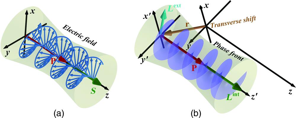
Fig. 1. Angular momentum in paraxial optical fields: (a) longitudinal SAM of the right-handed circularly polarized field and (b) intrinsic longitudinal OAM with the helical wavefront illustrated with the purple surface. An extrinsic OAM arises from a shift with respect to the coordinate systems.

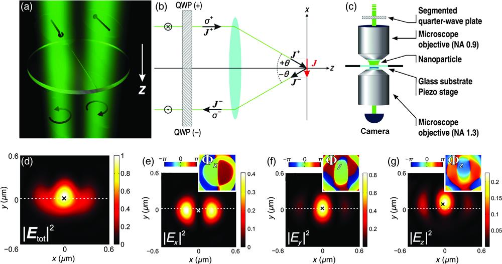
Fig. 2. Generation of the transverse SAM in highly confined field. (a) A segmented QWP is adopted to obtain the desired incident beam. (b) Schematic of tightly focusing the incident field. (c) The experimental setup to generate and characterize the transverse SAM of the focused field. The reconstructed distributions of |Etot|2, |Ex|2, |Ey|2, and |Ez|2 of the focal field are depicted in (d)–(g), respectively, and the insets present the corresponding relative phases. Panels (a)–(c) are reproduced with permission from Ref. 46; (d)–(g) are reproduced with permission from Ref. 72.

Fig. 3. Spin orientation control based on the time-reversal method. (a) Schematic of the inverse calculation method. The insets present the projections of the focal field on three orthogonal cross sections and its corresponding incident structured pupil field for θ1=π/6. (b) Evolution of the spin axis rotation in the yz plane. (c) The beam sizes of focal fields. Figure reproduced with permission from Ref. 75.

Fig. 4. Generation of the optical Möbius strip polarization topology. (a) Schematic of the experimental setup to tightly focus the optical fields generated from a q-plate. (b) Experimentally generated Möbius strip polarization topology with three half twists in the focal plane. (c) Experimentally measured Möbius strip polarization topology with five half twists in the focal plane. (d) Scattered fields from a silicon nanoparticle form a Möbius strip in any curve surrounding a C line. Panels (a)–(c) are reproduced with permission from Ref. 79. Panel (d) is reproduced with permission from Ref. 81.

Fig. 5. Generation of exotic optical Möbius strip polarization topology. (a) The intensity and polarization distributions in the pupil plane for the generation of an “8”-shaped twin Möbius strip. (b) Generation of an “8”-shaped twin Möbius strip in the focal area. The total intensity distributions in the focal plane with a prescribed “8”-shaped path denoted in the dashed black line. (c) The polarization topology along the red “8”-shaped path. (d) The intensity and polarization distributions in the pupil plane for the generation of a circular Möbius strip with changing twisting speed. (e) Generation of a circular Möbius strip with changing twisting speed in the focal region. (f) The two halves are plotted in red and black, respectively. The twisting rate of the black is twice that of the red half. Figure reproduced with permission from Ref. 82.

Fig. 6. STOV with transverse OAM. (a) Experimental generation based on an SLM and characterization based on interference with a femtosecond reference pulse. (b) Reconstructed spatiotemporal phase distribution. (c) Measured 3D iso-intensity profile of a spatiotemporal vortex of ℓ=1. (d) Measured 3D iso-intensity profile of a spatiotemporal vortex of ℓ=2. Figure reproduced with permission from Ref. 61.

Fig. 7. Ultrafast optical beams with time-varying OAM. (a) Two time-delayed, collinear pulses with different OAM values are focused into a gas target to produce self-torque beams. (b) Theoretical evolution of the intensity profile of the 17th harmonic at three temporal instants. (c) Evolution of the OAM of the 17th harmonic. (d) Interference fringe patterns of a chirped wave packet embedded with two spatiotemporal vortices with a short probe pulse. (e) 3D iso-intensity reconstruction of a wave packet containing two spatiotemporal vortices with temporal separation of 1 ps. Panels (a)–(c) are reproduced with permission from Ref. 91. Panels (d) and (e) are reproduced with permission from Ref. 93.

Fig. 8. Optical manipulation employing photonic AM. (a) Microscopic beads orbit in the optical vortex. (b) Metal particles manipulated with the PV tweezers. (c) Transverse spinning of a particle caused by the surface plasmonic field. (d) Schematic of enantioselective optical trapping with plasmonic tweezers. Panel (a) is reproduced with permission from Ref. 104, (b) is reproduced with permission from Ref. 105, (c) is reproduced with permission from Ref. 32, and (d) is reproduced with permission from Ref. 106.

Fig. 9. Spin-controlled directional coupling. (a) Asymmetric excitation of surface plasmon polariton wave. (b) Light with different polarizations coupled into a nanofiber via a nanoparticle. Experimental results of the scattered light at the right (c) and left (d) side of the nanofiber as a function of the nanoparticle position on the surface of the fiber and incident light polarization. Panel (a) is reproduced with permission from Ref. 108; (b)–(d) are reproduced with permission from Ref. 112.

Fig. 10. Optical communication using OAM of light. (a) Physical degrees of freedom of photons used in optical communication. (b) The schematic of optical communication between an UAV and a ground station utilizing OAM multiplexing. (c) OAM demultiplexing in a turbulent environment based on the SMART technique. Panel (a) is reproduced with permission from Ref. 117, (b) is reproduced with permission from Ref. 127, and (c) is reproduced with permission from Ref. 129.