
Zishuai Zeng, Zihao Pang, Keming Pan, Jia Xu, Daomu Zhao. Multiplication and division of orbital angular momentum beams by Fermat’s spiral transformation[J]. Photonics Research, 2023, 11(2): 165
- Photonics Research
- Vol. 11, Issue 2, 165 (2023)
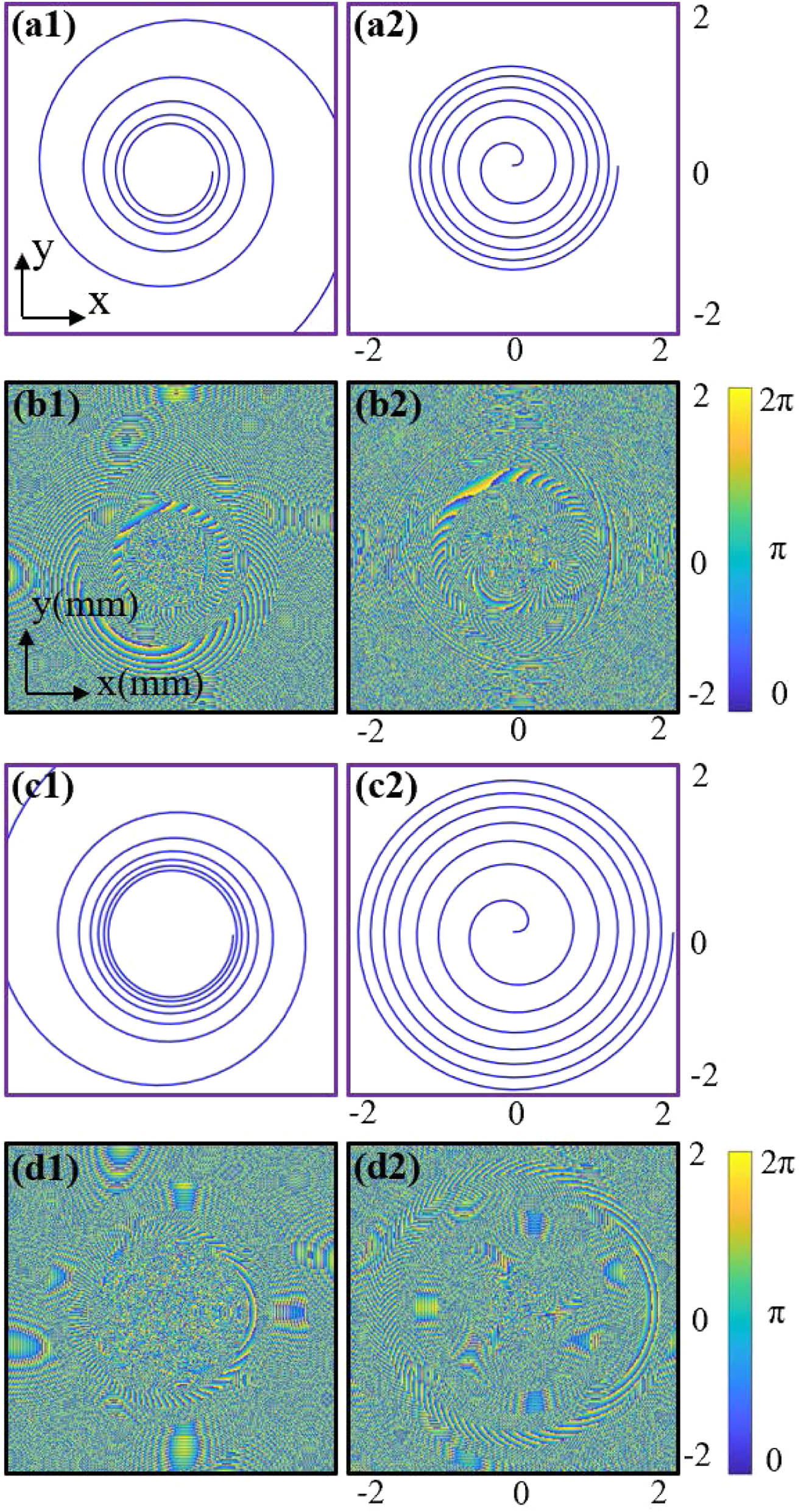
Fig. 1. Schematic illustration of Fermat’s spiral. (a), (c) Geometric pattern. (b), (d) Phase distribution. (a1), (b1) Transformation phase and (a2), (b2) correction phase with n = 8 / 5 n = 4 / 5
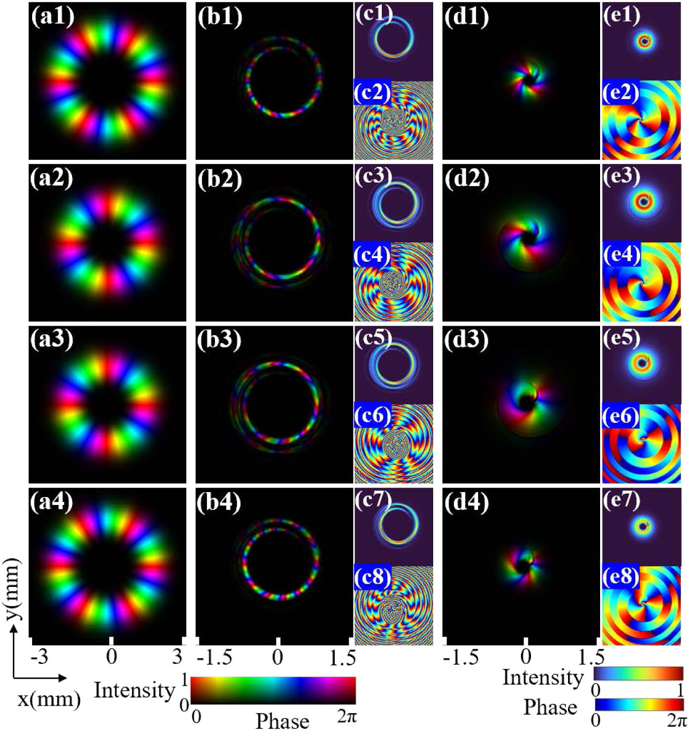
Fig. 2. Numerical simulations of Fermat’s spiral transformation on vortex beams in the case of integer multiplication and division. (a) Input LG beams with ℓ = − 6 , − 4 , + 4 , + 6 n = 2 n = 1 / 2
Fig. 3. Numerical simulations of Fermat’s spiral transformation on vortex beams in the case of fraction multiplication and division. (a) Input LG beams with ℓ = − 3 , + 3 , − 6 , + 6 n = 5 / 3 n = 2 / 3
Fig. 4. Phase with different transformation parameters n 2 and 3 . (a1)–(d1) Transformation phase. (a2)–(d2) Correction phase. (a1), (a2) n = 2 n = 1 / 2 n = 5 / 3 n = 2 / 3
Fig. 5. Power weight of the output OAM modes. (a) Multiplication with n = 2 n = 1 / 2
Fig. 6. Optical description of integer multiplication with n = 2 ℓ = − 3 , + 2 , + 3 , + 4 ℓ = − 6 , + 4 , + 6 , + 8
Fig. 7. Optical description of integer division with n = 1 / 2 ℓ = − 6 , + 4 , + 6 , + 8 ℓ = − 3 , + 2 , + 3 , + 4
Fig. 8. Optical description of fraction multiplication with n = 3 / 2 n = 3 / 4 ℓ = − 4 , − 6 , + 8 , + 12 ℓ = − 6 , − 9 , + 6 , + 9
Fig. 9. Schematic of the experimental setup. HP, half-wave plate; Pol.1–Pol.3, polarizer; × 10 × 10 NA = 0.25
Fig. 10. Evolution of input LG beams carrying ℓ = 4 n = 2 n = 1 / 2
Fig. 11. Evolution of input LG beams carrying ℓ = 5 n = 8 / 5 n = 4 / 5

Set citation alerts for the article
Please enter your email address
© Copyright 2018-2021 | Chinese Laser Press. All Rights Reserved 沪ICP备15018463号-20