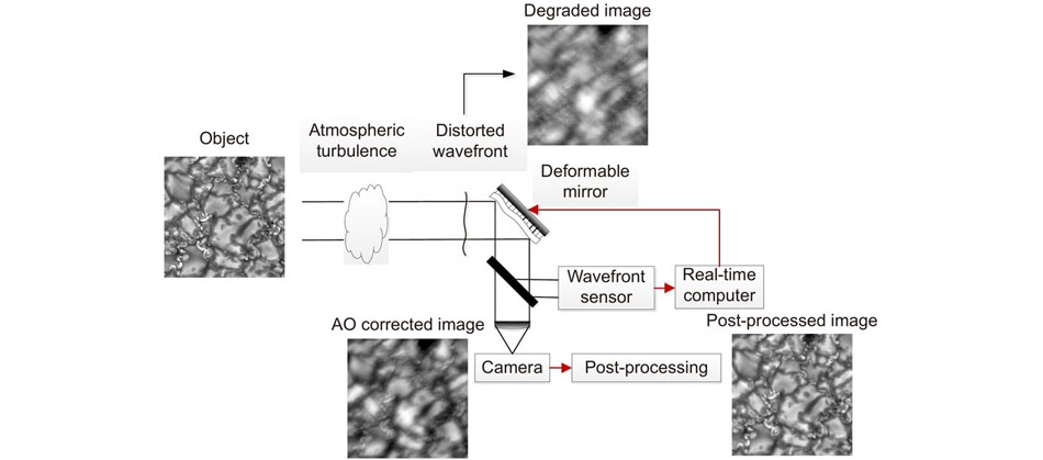
Fig. 1. Overview of AOS for solar observation. The light waves emitted by the Sun suffer from wavefront distortion when pass through the atmospheric turbulence. The WFS detects the intensity distributions caused by the wavefront distortion and then transfers them to the RTC. The RTC reconstructs the wavefront and calculates the voltages sent to the DM to compensate the distorted wavefront. Meanwhile, the scientific camera records the corrected images and sends them for post-processing in order to get even higher resolution.

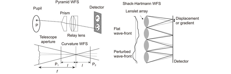
Fig. 2. Principles of three kinds of WFS. Figure reproduced with permisson from ref.³², Annual Reviews Inc.

Fig. 3. (a) The training algorithm of the ANN where displacements of the spots are taken as the inputs while the Zernike coefficients as outputs. To make the network more insensitive to the noise in the spot patterns, the training is also performed on noisy patterns. The noise added to the spot displacements follows Gaussian distribution. (b) The average reconstructed errors of ANNs with different number of neurons in the hidden layer shows that hidden layer with 90 neurons performs best. (c) Comparison of residual errors of LSF, SVD and ANN algorithms. Figure reproduced from ref.⁷¹, Optical Society of America.

Fig. 4. (a) The classification network similar to CoG method for spot detection with 50 hidden layer neurons named as SHNN-50. (b) The classification network with 900 hidden layer neurons named as SHNN-900. The input is the flattened subaperture image (25×25) and the output is a kind of classification in 625 classes, the same as the number of pixels indicating the potential center of the spot. Figure reproduced from ref.⁷³, Optical Society of America.

Fig. 5. (a) The architecture of the CNN for SHWFS. The input is a SHWFS image and the output is a vector, which indicates centroids. (b) The performance of CNN compared with MLP where the error is calculated as the average of the absolute value of the difference between all the output network centroids and the simulated true centroids. Figure reproduced from: (a, b) ref.⁷⁴, International Conference on Hybrid Artificial Intelligence Systems.

Fig. 6. (a) Architecture of ISNet. This network takes three 16×16 inputs (x-slopes, y-slopes and intensities) and outputs a 32×32 unwrapped wavefront. (b) Plot of average Strehl ratio vs. Rytov number for different reconstruction algorithms. For comparison, the Strehl ratio of a Marèchal criterion-limited beam is shown in (b), which is 0.82. Figure reproduced from: (a, b) ref.⁷⁵, Optical Society of America.

Fig. 7. Architecture of LSHWS. The network contains five convolutional layers and three full connected layers.The input is a SHWFS image of size 256×256. The output is a vector of size 119, which represents Zernike coefficients. Figure reproduced from ref.⁷⁶, Optical Society of America.

Fig. 8. (a) Architecture of SH-Net. The input is a SHWFS image of size 256×256, and the output is a phase map with the same size as the input. (b) the Residual block. ‘N’ and ‘N/4’ indicate the number of channels. (c) Statistical results of RMS wavefront error of five methods in wavefront detection. Figure reproduced from: (a–c) ref.⁷⁷, Optical Society of America.

Fig. 9. Architecture of the deconvolution VGG network (De-VGG). The De-VGG includes convolution layers, batch normalization layer filters, activation function ReLU, and deconvolution layers. The fully connected layers are removed, as the high output order slows down the calculation speed, but the deconvolution layer will not. Figure reproduced from ref.⁸⁰, under a Creative Commons Attribution License 4.0.

Fig. 10. (a) The data flow of the training and inference processes. (b) Strehl ratio of CNN compensation under different SNR conditions. Figure reproduced with permission from: (a, b) ref. ⁸¹, Elsevier.

Fig. 11. (a) The experiments of training and testing processes and inference acceleration. During training and testing processes, two networks were used, phase-diversity CNN (PD-CNN) and Xception. PD-CNN includes three convolution layers and two full connection layers. For each network, three sets of comparative experiments are set as following, inputting the focal and defocused intensity images separately, and inputting the focal and defocused intensity images at the same time. During the inference acceleration process, the trained model is optimized by TensorRT. (b) The inference time before and after acceleration with NVIDIA GTX 1080Ti. Figure reproduced from: (a, b) ref.⁸², under a Creative Commons Attribution License 4.0.

Fig. 12. Schematic and experimental diagram of the deep learning wavefront sensor. LED: light emitting diode. P: Polarizer. SLM: Spatial light modulator. DO: Dropout layer. FC: full connection layer. Figure reproduced from ref.⁸³, Optical Society of America.

Fig. 13. (a) Network diagram for CARMEN. where the inputs are the slopes of off-axis WFSs and the outputs are the on-axis slopes for the target direction. One hidden layer with the same number of neurons as the inputs is used to link the inputs and outputs and the sigmoid activation function is used. (b) On-sky Strehl ratio (in H-band) comparison with different methods. This on-sky experiment was carried out on the 4.2m William-Herschel Telescope. The Strehl ratios achieved by the ANN (CARMEN), the Learn and Apply (L&A) method and two GLAO night performances are compared. Figure reproduced from (a, b) ref.⁸⁴, Oxford University Press.

Fig. 14. Wind jumps of 7 m/s showing the convergence of the recursive LMMSE (blue) and the forgetting LMMSE (black), as well as the resetting of the batch LMMSE (green) for a regressor with a 3-by-3 spatial grid and five previous measurements for each phase point. Figure reproduced from ref.⁸⁷, Optical Society of America.

Fig. 15. (a) Robustness of the predictor against wind speed fluctuations between 10 and 15 m/s every 10 frames. (b) Robustness of the predictor against wind direction fluctuations between 0 and 45 degrees every 10 frames. Figure reproduced from: (a, b) ref.⁹¹, Oxford University Press.

Fig. 16. (a) Architecture of the encoder-decoder deconvolution neural network. The details of the architecture are described in Ref.⁹⁵. (b) Upper panel: end-to-end deconvolution process, where the grey blocks are the deconvolution blocks described in the lower panel. Lower panel: internal architecture of each deconvolution block. Colors for the blocks and the specific details for each block are described in the reference. Figure reproduced from: (a, b) Ref.⁹⁵, ESO.

Fig. 17. Top panels: a single raw image from the burst. Middle panels: reconstructed frames with the recurrent network. Lower panels: azimuthally averaged Fourier power spectra of the images. The left column shows results from the continuum image at 6302 Å while the right column shows the results at the core of the 8542 Å line. All power spectra have been normalized to the value at the largest period. Figure reproduced from ref.⁹⁵, ESO.

Fig. 18. The flowchart of AO image restoration by cGAN. The whole network consists of two parts, generator network and discriminator network, which are used for learning the atmospheric degradation process and achieving the purpose of generating restored images. The loss function of the network is a combination of content loss for generator network and adversarial loss for discriminant network. Figure reproduced from ref.⁹⁶, SPIE.

Fig. 19. The results of blind restoration for the Hubble telescope. (a) The sharp image, (b) the blurred image by Zernike polynomial method in atmospheric turbulence strength D/r₀= 10, and (c) the result of restoration by cGAN, respectively. Figure reproduced from ref.⁹⁶, SPIE.

Fig. 20. Block diagrams showing the architecture of the network and how it is trained by unsupervised training. Figure reproduced from ref.⁹⁷, arXiv.

Fig. 21. Original frames of the burst (upper row), estimated PSF (middle row) and for the GJ661.The upper row shows six raw frames of the burst. The second row displays the instantaneous PSF estimated by the neural network approach. The last row shows the results from re-convolve the deconvolved image with the estimated PSF. Figure reproduced from ref. ⁹⁷, arXiv.

Fig. 22. Controller for an AOS. (a) PI control model; (b) DLCM control model. ZA−1 and ZB−1 are the H-S sensor delay and control calculation delay, respectively. GWV (Generating wavefront to voltage). J and J0 are the cost functions of the network and the red dotted line is a gradient data stream. Figure reproduced from ref.¹⁰⁴, Optical Society of America.

Table 0. The detection speed of five methods. Table reproduced from ref.⁷⁷, Optical Society of America.

Table 0. The correlation coefficient of SHWFS patterns and the Strehl ratio of PSFs. Table reproduced from ref.⁷⁶, Optical Society of America.

Table 0. The inference time of De-VGG compared with SPGD. Table reproduced from ref.⁸⁰, MDPI.

Table 0. The false rate of different methods in low SNR situations, where CoG means Center of Gravity method and TmCoG means a modified CoG method using m % of the maximum intensity of spot as threshold. Table reproduced from ref.⁷³, Optical Society of America.

Table 0. Summary of accuracies (RMSE:λ) of Zernike coefficients estimated by Xception. Table reproduced from ref.⁸³, Optical Society of America.

Table 0. Summary of accuracies (Root Mean Square Error (RMSE):λ) of Zernike coefficients estimated by PD-CNN. The focal model and defocused model mean the input of PD-CNN is a single focal intensity image or defocused intensity image. The PD model means that the input of PD-CNN includes both focal and defocused image. Table reproduced from: (a, b) ref.⁸², MDPI.

Table 0. The general information and differences of all the four networks.