Adaptive optics (AO) is a dynamic wavefront compensation technique widely used in various applications such as ground-based telescopes^{1, 2}, laser communication³, and biological imaging^{4, 5} et al. In astronomy, almost all of the ground-based high-resolution imaging telescopes with apertures larger than 1m have been equipped with AO systems (AOS). In microscopy, AO is becoming a valuable tool for high resolution microscopy, providing correction for aberrations introduced by the refractive index structure of specimens⁶. In quantum communication, AO is used to compensate the effects of atmospheric distortion to maximize the quality of the optical link and reduce the turbulence induced loss and noise at the receiver⁷. In 2019, the Air Force Research Laboratory Starfire Optical Range demonstrated that quantum communication with AO can support the quantum communication through-the-air in daylight under conditions representative of space-to-Earth satellite links⁸. In retinal imaging, AO is being used to enhance the ability of optical coherence tomography, fluorescence imaging, and reflectance imaging⁹.

Our laboratory, the key laboratory on AO in Chinese Academy of Sciences is one of the largest teams in the world working on AO which has the capability to develop the complete set of AOS. We apply AO techniques to astronomical telescope^10-12, inertial confinement fusion¹³, space-to-earth laser communication¹⁴, retinal imaging¹⁵ et al. Here brief introduction of some recent developments in the laboratory is presented. In astronomical observation, we did the first on-sky demonstration of piezoelectric adaptive secondary mirror based AOS in 2016¹⁶. We built and successfully tested the first multi-conjugate AO (MCAO) system in China on the 1-m New Vacuum Solar Telescope in 2017¹⁷. We also built one of the largest solar telescopes in the world, the 1.8-m Chinese Large Solar Telescope equipped with a 451-unit AOS and the telescope saw its first light in 2020¹⁸. In free-space laser communication, an experiment of a 5-Gbps free-space coherent optical communication system was finished with bit-error rate under 10^–6 after AO compensation¹⁹. Besides, different kinds of deformable mirrors have been developed and used in different areas²⁰.

Although AO has been already successfully implemented in many areas to improve the image resolution or peak energy of lasers, there are still some challenging problems. For example, how to get the wavefront of wavefront sensor less (WFS-less) AOS²¹ or array telescopes with high speed, how to estimate the wavefront along the line of sight to the scientific target in multi-object AO (MOAO) system²² and how to reduce the time-delay error in extreme AOSs²³, etc. With the development of machine learning, especially the deep learning techniques²⁴, some of these complex or inverse problems can be solved. Machine learning is a concept that an algorithm can learn and adapt to new data without human intervention. It is usually divided into two kinds of methods, supervised learning and unsupervised learning. Supervised learning is provided with training data containing not only inputs but also outputs that are also named as labels. The most popular collection of supervised learning algorithms is deep learning which is composed by multiple layers of neural networks. In general, at least three important tasks in AO require such tools including determining the aberration from optically modulated images in WFS, predicting future wavefront with historical multi-source information and reconstructing the high-resolution images from the noisy and blurred ones. These problems are either ill-conditioned or highly nonlinear. Typical traditional algorithms such as least square fit (LSF), singular value decomposition (SVD), or Gauss-Seidel et al. either have weak fitting capability or require many iterations. On the contrary, deep learning algorithms not only have strong fitting capabilities but also can contain the prior information in the network’s structure and weights. These natures can help AO solve the above problems. Besides, the structure of AOS may be also simplified by the powerful algorithms and computation.

Machine learning in AO was investigated as early as 1990 s^25-27. At that time, artificial neural networks (ANN) were considered to be a good alternative for the wavefront sensing of single-aperture and array telescopes in the multiple mirror telescope (MMT)²⁸. Experiment has been done on the MMT to demonstrate the advantages of the ANN²⁹. The same technique was used to estimate the aberration of Hubble space telescope and got almost the same result of slow off-line Fourier based phase-retrieval methods³⁰. Meanwhile, the prediction of turbulence with ANN was also studied and some simulation results showed potential superiority³¹.

With the fast development of deep learning algorithms, computation power and explosive expansion of data, we have already seen great advancements in computer vision, speech recognition and natural language processing, etc. In recent years, rapidly growing number of researches working on machine learning-assisted intelligent AO (IAO) have been published and more are expected in the near future. In this review, recent advancements on IAO are summarized and future development trends are discussed. This review is organized as follows. Traditional AO is briefly introduced in Section Brief introduction of adaptive optics system, IAO including the intelligent wavefront sensing, intelligent wavefront prediction, intelligent post-processing as well as other applications are described in Section Intelligent adaptive optics, and finally in Section Conclusion &discussion, we draw the conclusion and discuss the future development of IAO.

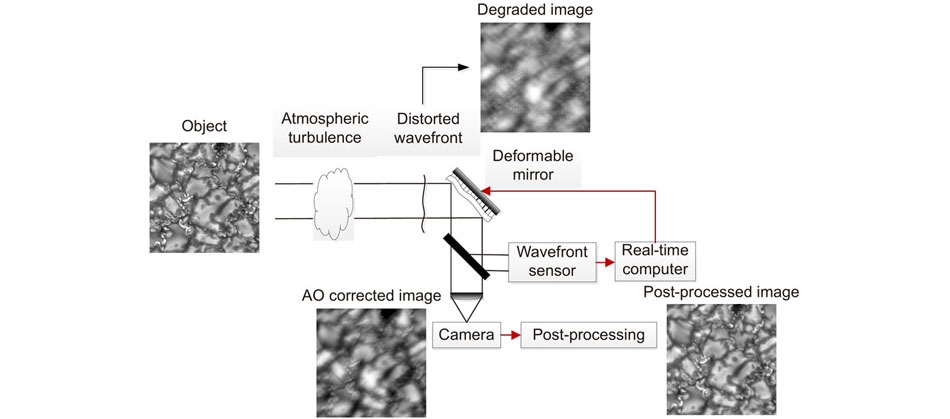
Taking the solar observation as an example, the AOS is basically composed of a deformable mirror (DM), a WFS, a real-time controller (RTC), and a post-processing program, as described in Fig. 1.

Wavefront sensing is a technique to provide a signal with which the shape of the wavefront can be estimated with sufficient accuracy³². Several kinds of WFSs are frequently used in different AOSs including the Shack-Hartmann WFS³³ (SHWFS), Pyramid WFS³⁴ and curvature WFS³⁵ as shown in Fig. 2. These traditional WFSs build linear relationship between the wavefront and the selected features such as sub-aperture slopes, wavefront curvatures or image intensity differences. On one hand, owing to the simple relationship, wavefront can be reconstructed quickly enough to satisfy the millisecond time-scale speed required by the AOS. On the other hand, these WFSs have complex optical setup and require high accuracy alignment. Besides, some demands such as continuous wavefront or uniform amplitude must be met for these gradient or curvature-based methods. These requirements can be broken in some extreme observation circumstances when the target is at low-elevation or the turbulence is too strong and then the performance would deteriorate quickly.

Wavefront reconstruction and control builds the relationship between DM commands and the WFS measurements. The wavefront here can be represented as a 2-dimensional phase map as well as modal coefficients of some bases such as the Zernike modes³⁶, Karhunen–Loève modes³⁷ or the so-called Nodal modes³⁸. The wavefront reconstruction spatially filters the WFS measurements and recovers the closed-loop wavefront error while the wavefront control temporally filters the wavefront error and drives the DM. The most popular control in AO is the class of proportional-integral-derivative (PID) algorithms including the integrator or the proportional-integral (PI) control et al³⁹. However, innumerable researches have shown that PID is not the optimal choice for AOSs, because its poor performance for the correction of dynamic turbulence and narrow-bandwidth disturbances. Linear quadratic Gaussian (LQG) control based on Kalman filter is an appealing control strategy^40-44. It can obtain an optimal correction in terms of residual phase variance by performing optimal prediction of dynamic disturbance. The key of this method is to quickly and consecutively build the accurate dynamical model to track the time-varying dynamic disturbance^{45, 46}. LQG is a kind of linear prediction algorithm in which any deviation from the estimated model would degrade the performance.

The AOS can only partially correct the distortions in real time due to the unavoidable inherent errors of the system. The residual errors which are composed by the measurement error, fitting error, time-delay induced error, and anisoplanatism error et al. decrease the quality of the imaging. Thus, post-facto processing techniques are required to reach diffraction limit of the system.

The image of the astronomical object i(x) can be expressed mathematically as the convolution of the object intensity o(x) and the point spread function (PSF) of the whole atmosphere + telescope + instruments system p(x):

1i(x)=o(x)*p(x).

In the Fourier domain the equation is transformed to

2I(v)=O(v)⋅P(v),

where the upper characters are defined as the Fourier transform of the lower cases, and v is the index at the frequency domain. To deconvolve the object intensity o(x) from the observed intensity i(x), the PSF of the system is needed. The precise PSF is rarely known in actual system, except that the residual wavefront is measured or there is an unresolved star within the isoplanatic angle. Thus, the blind deconvolution (BD)^47-49 is proposed using only the prior assumption of the system to simultaneously obtain the object and the PSF. The BD is ill-defined due to the deficiency of the information about the actual system and thus the accuracy of the reconstruction depends on the rationality of the assumed priors.

Another comparable method is the phase diversity (PD) method^50-52 which can be considered as a special case of the BD. With an additional information on the phase (usually using the defocus of one image), the method can detect the residual wavefront simultaneously and can be used for wavefront sensing in the AOS.

Adding more information of the system can lessen the ambiguity of the BD method and get more reliable result. The multi-frame BD (MFBD)^53-55 and the multi-object MFBD (MOMFBD)⁵⁶ are then introduced. By assuming the observed object is not changed during the time used to capture the multiple image frames, the solutions of the method are more robust than the BD. The MFBD is further extended to include the multiple objects case. The MOMFBD consists of a maximum-likelihood solution to the deconvolution problem which is widely used in the case of simultaneously reconstructing the broad-band and narrow-band channel images at the solar observations.

The statistical information of the turbulence can also be applied in the reconstruction of the astronomical object. The speckle imaging method uses the short exposure images to recover the Fourier amplitude and the Fourier phase of the object separately. In the process, the Fried parameter of the turbulence is estimated and the speckle transfer function of the system which is the power spectrum of the PSF is deduced using the correction abilities of the AOS and the Fried parameter of the turbulence^{57, 58}. The Labeyrie’s method is used to deconvolve the Fourier amplitude of the object⁵⁹. The triple-correlation bispectra method^60-62 and the Knox-Thompson cross-spectrum method⁶³ reconstruct the Fourier phase of the object. The reconstructed objects are obtained by inverse transforming the Fourier amplitude and the Fourier phases.

The high photometric accuracy of the MOMFBD method and speckle imaging method are confirmed by their wide applications on the reconstructions of the astronomical objects at nearly all the ground-based observation sites^64-67. But the drawbacks of those method are the necessary computing effort and memory for the masses of iterations within the process. To get a real time reconstruction, those methods usually require the use of a dedicated computer cluster or similar installations^{68, 69}. However, the processing time can be significantly decreased using the intelligent image reconstruction methods described in Subsection Intelligent adaptive optics.

AOS by its name has already shown some degree of intelligence. In this review, we distinguish the intelligence from non-intelligence by the application of machine learning techniques which can learn rules from data. IAO is a technique that reshapes the wavefront aberration measurement, control and post-processing through machine learning to improve the performance of AO or simplify the system complexity. Recent advancements in IAO are summarized in this section.

SHWFS is the most widely used WFS in AOS due to its simple structure, alignment and less computation. However, the reconstructed result is sensitive to noise. Besides of improving the measurement accuracy of SHWFS by optical modulation⁷⁰, advanced algorithms can also be used. Two kinds of machine learning-based methods are proposed to improve the SHWFS’s performance. One is to improve the gradient-based method such as building the relationship between aberrations and gradients with nonlinear fitting tools such as ANN instead of simple matrix multiplication, or improving the spot centroid accuracy by doing the spot classification with ANN before centroid calculation. The other is to extract the aberration from the SHWFS image directly with deep learning instead of calculating the gradients. In some applications, traditional special WFSs are not allowed and the imaging setup can be used as the PD WFS or single-image phase retrieval WFS. In these cases, deep learning can be used to solve the nonlinear phase retrieval problem without many iterations required by traditional Gauss-Seidel or stochastic parallel gradient descent (SPGD) methods etc. Besides of improving accuracy and speed of traditional narrow field-of-view WFS, deep learning can also be used to improve the performance of tomography WFS.

Generally, wavefront is calculated from sub-aperture spot displacements with LSF or SVD in SHWFS. Guo et al proposed to use ANN to reconstruct the wavefront from noisy spot displacements after comparing the performances of LSF, SVD and ANN. The lens array of the SHWFS was assumed to consist of 8×8 sublenses. Different structures of neural network were investigated to find the optimal network architecture. For training on the noisy patterns, the best network was a three-layer feed forward back-propagation network with 90 neurons in the hidden layer. The principle of training and simulation result are shown in Fig. 3. After training on the noisy patterns, the residual error of ANN is much smaller than the other two methods⁷¹. Besides of ANN, Swanson et al proposed to use a U-Net architecture to learn a mapping from SHWFS slopes to the true wavefront in 2018, but this method was not compared with others⁷².

To overcome the strong environment light and noise pollutions, Li et al. proposed another method based on ANN, namely SHWFS-Neural Network (SHNN), as described in Fig. 4. In this method, SHNNs firstly find out the spot center, and then calculate the centroid, which transform spot detection problem into a classification problem. As shown in Table 1, when the signal-to-noise ratios (SNRs) are interfered by the environment light and ramp in the subaperture images, SHNNs show stronger robustness compared with other methods, which means this method can be used in AOSs under extreme conditions⁷³.

To avoid any information loss during the centroid calculating procedure in off-axis WFSs, Suárez Gómez et al. presented a method using convolutional neural network (CNN) as a reconstruction alternative in MOAO⁷⁴. As displayed in Fig. 5(a), this method relies on the use of the full image as input, instead of only the centroids. Simulations have shown the advantages of CNN compared with the multi-layer perceptron (MLP) as shown in Fig. 5(b). The promising results of CNN open possibilities in further work in the topic, such as improving the topology of the network, setting more solid testing with sets of multilayer turbulence profiles and using optical measurements for the comparison of errors.

Although Suárez Gómez et al use the whole off-axis SHWFS images as input, they still calculate the slopes of the on-axis target and use these slopes to reconstruct the wavefront. However, calculating only the centroids or slopes dose not overcome the limitations of the wavefront reconstruction using slope features. To further improve the performance of SHWFS, DuBose et al.⁷⁵ extended the work of Swanson et al.⁷² and developed the Intensity/Slopes, or ISNet, a deep convolution network utilizing both the standard SHWFS slopes and the total intensity of each subaperture to reconstruct aberration phase. The architecture of the ISNet is shown in Fig. 6(a). The main difference between ISNet and the work of Swanson et al. is the use of intensity and dense blocks. Four reconstruction algorithms (ISNet, ISNet without intensity, Swanson et al.’s work and the Southwell Least Squares) are compared in ref.⁷⁵. The results are shown in Fig. 6(b). The ISNet offers superior reconstruction performance.

In biological applications, deep learning has been used to detect high-order aberration directly from SHWFS images without image segmentation or centroid positioning. Hu et al. proposed a method named learning-based Shack-Hartmann wavefront sensor (LSHWS) which could predict up to 120^th Zernike modes with a SHWFS image as input⁷⁶. The architecture of the LSHWS is displayed in Fig. 7. The compensation results of LSHWS and Traditional Shack-Hartmann wavefront sensor (TSHWS) are given in Table 2. The correlation coefficient of LSHWS corrected patterns is ~5.13% higher than that of TSHWS. In addition, Hu et al.⁷⁷ also proposed another deep learning assisted SHWFS named SH-Net which could directly predict the wavefront distribution without slope measurements or Zernike modes calculation. The architecture of SH-Net is shown in Fig. 8(a) and 8(b). The detection speeds of different methods are given in Table 3. From Fig. 8(c) and Table 3, we can see that SH-Net has the highest accuracy among the five methods. Although the detection speed of the SH-Net is slower than approach of Swanson et al. and zonal, the accuracy is much higher.

Compared with SHWFS, image-based wavefront sensing is a method without additional optical components but using parameterized physical model and nonlinear optimization. PD WFS is such a type of image-based WFS. As early as 1994, Kendrick et al. used general regression neural network to calculate the wavefront errors from focused and defocused images⁷⁸. Recently, with the development of artificial intelligence, many new methods based on CNN for wavefront detection have been proposed. J R. et al. used machine learning to determine a good initial estimate of the wavefront. Although it can improve the effectiveness of the traditional gradient descent algorithm, iterative operations are still required⁷⁹. Guo et al. used an improved CNN to successfully establish the nonlinear mapping between the focal/defocused PSFs and the corresponding phase maps⁸⁰. As shown in Fig. 9, their deconvolution visual geometry group network (De-VGG) adds three deconvolution layers on the basis of the well-known visual geometry group (VGG) network. Compared with SPGD algorithm, De-VGG has a great advantage in running time. The inference time of SPGD and De-VGG is shown in Table 4.

Ma et al. proposed a similar PD wavefront sensing technique to Guo et al.’s⁸⁰ meanwhile, as shown in Fig. 10⁸¹. There are two CCDs for detecting intensity images. The AlexNet is used to extract the features from the focal and defocused intensity images and obtain the corresponding Zernike coefficients. Figure 10(c) shows the Strehl ratio of CNN compensation under different SNR conditions. When the SNR reaches 50 or 35 dB, the compensation results are almost coincided and the system is robust. When the SNR reaches 20 dB, the robustness of the system reduces and the results fluctuate greatly. As no real data or experiments were used to investigate the accuracy, it is not clear about the robustness of this method.

Wu et al. proposed a novel real-time non-iterative phase-diversity wavefront sensing based CNN that achieves sub-millisecond phase retrieval⁸². Figure 11 shows two parts of the experiments. This method improves the real-time performance by using NVIDIA TensorRT (an SDK for high-performance deep learning inference) and reduces the aberration measurement error by fusing the focal and defocused intensity images. However, there is some accuracy loss after inference acceleration (Table 5). It is necessary to further study hardware optimization principles of TensorRT.

To further simplify the optical setup, Nishizaki et al. proposed a variety of image-based wavefront sensing architectures named deep learning WFS (DLWFS) that could directly estimate aberration from single intensity image using Xception⁸³. As shown in Fig. 12, this method is suitable for both point and extended sources and the types of preconditioners include overexposure, defocus and scatter. The results in Table 6 show that all of the mentioned preconditioners can vastly improve the estimation accuracy when performing in-focus image-based estimation and among them overexposure is the optimal. For further study, it is important to compare the DLWFS with conventional WFSs to validate its usefulness as a practical replacement.

Traditional single conjugate AOS can only work when the scientific target is near a bright guide star or the scientific target itself is bright enough. These requirements limit the number of stars on the sky that can be observed with high resolution. The majority of modern AOSs use tomographic reconstruction techniques to overcome this problem. The mostly investigated configurations are laser tomography AO, MCAO and MOAO.

MOAO is a large-field-of-view AO technique which simultaneously measures the open loop wavefront of several distributed guide stars and estimates the phase aberration of each target. Osborn et al. proposed a MLP named CARMEN to combine the information from the off-axis WFS slopes and output the on-axis wavefront slopes from the target to the telescope⁸⁴. The MLP diagram and experimental result of CARMEN are shown in Fig. 13. As demonstrated by the results, the L&A tomographic reconstruction outperforms the CARMEN by approximately 5% in Strehl ratio. However, CARMEN is considered to be more robust when the altitude of high layer turbulence changes because in L&A, the on-line measurements from all of the WFSs must be combined and theoretical functions are used to recover the turbulence profile. Moreover, the experiment also proved that off-line training using simulation data can be used for realistic situations.

Due to the exposure and readout time required by the WFS, the reconstruction and control calculation time cost by the RTC and the response time of the DM, AOS usually suffers about 2~3 frames time delay. Traditional control algorithms don’t consider the wavefront distortion change from measurement to correction so there is a so-called time-delay error. One of the effective methods to reduce this time-delay error is to predict the future wavefront with several previous frames.

As firstly demonstrated by Jorgenson and Aitken that astronomical wavefront can be predicted⁸⁵, numerous efforts have been done to improve the prediction accuracy. At first, linear predictors such as the linear minimum mean square error (LMMSE) algorithm based on the statistical knowledge of the atmosphere, noise etc. were investigated, with the advantages of simple architecture and less computations⁸⁶. However, the accurate a priori knowledge about the atmospheric turbulence and noise cannot be obtained easily in real systems, especially for non-stationary turbulences. For instance, as shown in Fig. 14, the varying wind speed has a significant impact on the performance of prediction, preventing it from reaching optimal performance⁸⁷.

Two classifications of algorithms are expected to solve this problem, one is to estimate the statistical properties in quasi real-time⁸⁸ and the other is to train the predictor with big data to adapt the variation of the turbulence. The machine learning based predictor belongs to the second one. As early as 1997, Montera et al compared the LMMSE estimator with neural network estimator and drew the conclusion that the neural network could outperform the LMMSE when the seeing varies over a range of conditions³¹. Early studies about prediction using neural networks were usually based on the feed-forward MLP network. With the development of deep learning, recurrent neural networks having dynamic feedback connections and sharing parameters across all time steps are better for sequence data processing tasks like wavefront prediction. Long short term memory (LSTM) has been extensively studied to predict the turbulence induced wavefront^{72, 89, 90}. As shown in the Fig. 15, Liu et al. showed that LSTM had the ability to learn information such as wind velocity vectors from the data and could use this information for prediction in open-loop AOS⁹¹. Liu emphasized that the selection of training regime was very important for the performance of ANN’s prediction. This means that the training data and methods play a great role in machine learning-based prediction. To fight against overfitting and improve the generalization capability, Sun et al. proposed a Bayesian regularization back propagation algorithm to make the tradeoff between the fitting error and model complexity in the objective function⁹².

It can be anticipated that the prediction of atmospheric distorted wavefront will be a research focus in the near future especially for high contrast AO⁹³ and low-flux AO⁹⁴. Deep learning techniques have superior advantages over linear predictors when dealing with real non-stationary turbulence. However, several problems have to be analyzed and tested before applying in real AOS. One is the impact of error introduced by additional noise and nonlinear response of the system on prediction accuracy when pseudo open-loop slopes have to be used in real closed-loop AOS. Another is the trade-off between prediction accuracy and calculation amount for real-time operation of the RTC. Besides, the most important task for machine learning-based prediction algorithm development seems to collect enough high-quality training data for better generality of working with real time-varying turbulence. Whether simulated data can be used to train predictors used on-sky is worth studying.

One attractive advantage of the machine learning technique is the rapid processing rate once the model is trained. In the reconstruction of the astronomical objects, machine learning can dramatically decrease the computing time compared with traditional methods. With suitable computer hardware, it is anticipated that on-site real-time reconstruction of astronomical images will be possible in the near future.

Based on the theoretical basis of the MFBD, two different deep learning architectures were proposed by Ramos et al. in 2018⁹⁵, which are shown in Fig. 16. The first one (Fig. 16(a)) fixes the number of inputting frames and uses them as channels in a standard CNN which is an end-to-end approach based on an encoder-decoder network. The output of the CNN is the corrected frame, taking into account all the spatial information encoded in the degraded frames. To process a larger number of frames, one applies the deep neural network (DNN) in batches until all frames are exhausted. The second approach (Fig. 16(b)) uses a DNN with some type of recurrence, so that frames are processed in order. New frames are injected on the network and a corrected version of the image is obtained at the output. Introducing new frames on the input will slowly improve the quality of the output. This procedure can be iterated until a good enough final image is obtained. Both methods use the supervised learning where the training data is labeled by the corresponding MOMFBD result.

Figure 17 shows that both of the recurrent and encoder-decoder architectures are able to recover spatial periods between ~3 and ~30 pixels and increase their power, imitating what is done with MOMFBD. However, there is an apparent lack of sharpness and a slightly decrease of the power spectrums in the output of the networks compared with results of the MOMFBD in ref.⁹⁵. The authors thought that part of the sharpness in the MOMFBD image was a consequence of the residual noise. The random selection of patches for building the training set has the desirable consequence of breaking a significant part of the spatial correlation of the noise in the MOMFBD images. Consequently, the networks are unable to reproduce it and, as a result, partially filter it out from the prediction. Thus, high photometric accuracy reconstructions can be obtained even when the images are degraded by noise. Furthermore, the architectures significantly accelerate the BD process and produce corrected images at a peak rate of ~100 images per second.

As both methods mentioned use the training data labeled by the corresponding MOMFBD result, the precision of the net depends on the photometric accuracy of the MOMFBD method. The supervised manner also limits its application in other areas. Besides, the loss functions are the l₂ distance between the deconvolved frames obtained at the output of the network and the one deconvolved with the MOMFBD algorithm. It is known that the l₂ norm of the residual tends to produce fuzzy reconstructions, especially when the number of frames is small. Those aspects can be improved in the future research of image reconstruction.

Another supervised manner deep learning architecture was proposed by Shi et al in 2019⁹⁶. The authors proposed an end-to-end blind restoration method for ground-based space target images based on conditional generative adversarial network (cGAN) without estimating PSF. The flowchart of the model is displayed in Fig. 18. The training dataset of this network contains 4800 frames of simulated AO corrected space targets.

Figure 19 displays the reconstructed result of the Hubble telescope with cGAN. It could be seen that the quality of the restored image is improved. It not only accurately recovers the geometric contour of the image but also has remarkably improved some high-frequency details. The processing rate accelerates more than 100 times over traditional methods. Experimental results demonstrate that the proposed method not only enhances the restoration accuracy but also improves the restoration efficiency of single-frame object images at relative worse atmospheric conditions. Those improvements may be due to the improved loss function of this network. As no real space target images are used to validate the accuracy of the architecture, it is not clear about the robustness of this method.

The two methods above are based on the supervised manner and no information about the residual wavefront can be obtained in those procedures. In 2020, A. Asensio Ramos proposed an unsupervised method which can be trained simply with observations⁹⁷. The block diagrams shown in Fig. 20 display the architecture of the network. The authors proposed a neural network model composed of three neural networks which are trained end-to-end. In the model, the linear image formation theory is introduced to construct a physically-motivated loss function. The analysis of the trained neural model shows that MFBD can be done by self-supervised training, i.e., using only observations. The outputs of the network are the corrected images and also estimations of the instantaneous wavefronts.

The training set consists of 26 bursts of 1000 images each with an exposure time of 30ms, enough to efficiently freeze the atmospheric turbulence. The images are taken at different times, and cover reasonably variable seeing conditions. Given the unsupervised character of the approach, the neural network can be easily refined by adding more observations which can cover different seeing conditions. Figure 21 displays the results of the method at the GJ661 object. The results of this operation are similar to the observed frames, apart from the obvious noise. It is obvious from the deconvolved images that the individual estimated wavefronts agree to some degree with the real ones.

The network model is on the order of 1000 times faster than applying standard deconvolution based on traditional optimization. With some work, the model can be used in real-time at the telescope. Given the lack of supervision, the method can be generally applied to any type of objects, once a sufficient amount of training data is available. Further improvement can be done by adding more training examples with a larger variety of objects, from point-like to extended ones.

The general information and differences of all the four networks described above are summarized in Table 7.

There are also some instructive researches on image deblurring and reconstruction including enhancing the SDO/HMI images using deep learning⁹⁸, spatio-temporal filter adaptive network for video deblurring⁹⁹ and the deblurring of AO retinal images using deep CNNs¹⁰⁰ etc. All the methods show wonderful outcomes at specific domain but the robustness of the architectures is doubtful. The accuracy is highly dependent on the independent identically distributed property of the training data and the test data. At the most time, the degraded procedures of the images observed by the ground-based telescopes are random and uncertain. That’s why the deep learning reconstruction methods are not widely used by the astronomers until now. Training none end-to-end network and combining it with the imaging theory of the system may facilitate the applications of the machine learning in the post processing field.

WFS-less AO is a type of AOS where no specific WFS is used. The WFS-less AO mainly has two approaches: model-free and model based. Model-free approach, such as SPGD¹⁰¹, is based on blind-optimization and its convergence speed is slow. The model-based approach is based on the approximately linear relation between the aberration features and the far-field intensity distribution features. Those features are designed by experts in the field. However, the linear relationship and feature optimality are often questionable. To solve the above problems, Hu proposed a self-learning control framework for WFS-less AOS through deep reinforcement learning¹⁰². The aberration correction process is expressed as a Markov decision process, which is represented by a 5-tuple (S, V, P, R, γ): a state space S, an action space V, a state transition probability P(St+1|St,Vt): a reward function R(s, v), and a discount factor γ( γ∈[0,1])¹⁰³. Compared with the model-free method, the deep learning method accelerates the convergence by the gained experience of value function. On the other hand, compared with the model-based method, a deep learning network extracts the features of the far field raw images and the deterministic policy gradient network can deal with the nonlinear relationship between extracted features.

In order to cope with the disturbance of slope response matrix and improve the adaptive ability of AO control system, Xu proposed a deep learning control model (DLCM)¹⁰⁴. The PI and the DLCM control models are shown in Fig. 22.

The DLCM consists of a model net and an actor network. The model network and actor network have the same structure but have different roles. The model network shares the trained parameters with the actor network to stabilize the output of the actor network and improve the convergence speed of the actor network. The actor network updates the decision sample space and guides the update of the model network. Furthermore, compared to the fixed parameter PI control, real-time update of the actor network can cope with the disturbance of slope response matrix and improve control accuracy of the DLCM.

Recent advances in IAO are summarized including the intelligent wavefront sensing, wavefront reconstruction and control as well as post-processing. By using the machine learning, a lot of inverse or complex problems can be solved if large-scale datasets are available. Two main scenes seem to be particularly suitable to use machine learning at present. One is to use the ANN to build the relationship between the measurement (image) and the wavefront for wavefront reconstruction or the relationship between blurred image and the diffraction-limited image for post-processing. On one hand, features extracted from data may perform better than the manually selected linear ones. On the other hand, some iterative methods for phase retrieval may be replaced by deep learning for faster speed. The other is to use the ANN to do the nonlinear wavefront prediction for better accuracy and more importantly to adapt to the non-stationary turbulence.

Besides of the algorithms, the large-scale and high-quality data is also important which may be not easy to get. Some data can be generated by the computer for the training but its adaptability to the real systems needs to be demonstrated. Although lots of simulation and laboratory results have been obtained, less have been used in real AOSs recently. The application of IAO in real system is of great importance for demonstrating the generalization ability and real-time performance. As long as an on-sky demonstrator succeeds, lots of great progresses can be expected. In the more distant future, with the development of unsupervised learning and reinforcement learning, we can imagine an IAO system that can keep learning the rules from on-line multisource data to improve itself.