• Photonics Research
  • Vol. 11, Issue 1, 81 (2023)
Yihong Zhang, Wenjun Yu, Pei Zeng, Guoding Liu, and Xiongfeng Ma*
Author Affiliations
  • Center for Quantum Information, Institute for Interdisciplinary Information Sciences, Tsinghua University, Beijing 100084, China
  • show less
    DOI: 10.1364/PRJ.473970 Cite this Article Set citation alerts
    Yihong Zhang, Wenjun Yu, Pei Zeng, Guoding Liu, Xiongfeng Ma. Scalable fast benchmarking for individual quantum gates with local twirling[J]. Photonics Research, 2023, 11(1): 81 Copy Citation Text show less
    Illustrations of circuit and procedures used in (a) CCB and (b) CAB protocols. The orange boxes represent the target gate U and its inverse gate U−1. The blue and green boxes represent the random Pauli gate and random local Clifford gate. The yellow boxes denote the inverse gate for the m inner gate layers in the light blue box. Here, Pk(i) is a single-qubit Pauli gate on qubit k, and P(i)=P1(i)⊗⋯⊗Pn(i) is an n-qubit Pauli gate.
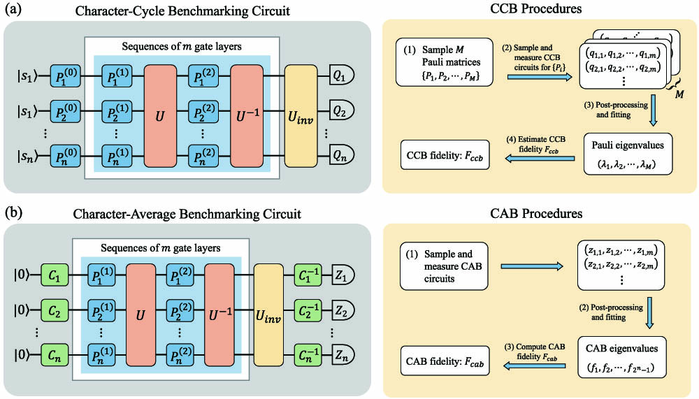
    Fig. 1. Illustrations of circuit and procedures used in (a) CCB and (b) CAB protocols. The orange boxes represent the target gate U and its inverse gate U1. The blue and green boxes represent the random Pauli gate and random local Clifford gate. The yellow boxes denote the inverse gate for the m inner gate layers in the light blue box. Here, Pk(i) is a single-qubit Pauli gate on qubit k, and P(i)=P1(i)Pn(i) is an n-qubit Pauli gate.
    Illustrations of the noisy CCB circuit with local gauge transformation. For simplicity, we show the case that the local gates are noiseless. The grey dashed boxes denote the noise channel Λ. The orange boxes represent the target gate U and its inverse gate U−1. The blue boxes represent the random Pauli gates. The green boxes represent the inserted local gates L and L−1, where L=⊗i=1nLi. The yellow box denotes the inverse gate for the m inner gate layers in the light blue boxes. In practice, we implement gates in circuit (b) while absorbing local gates L and L−1 into twirling and target gates. Here, the target gate following gauge transformation becomes LUL−1. Note that circuit (a) is equivalent to a CCB circuit with target gate U and noise channel ℒ−1Λℒ. Thus, it can be implemented to estimate Fccb(ℒ−1Λℒ), which is close to F(Λ).
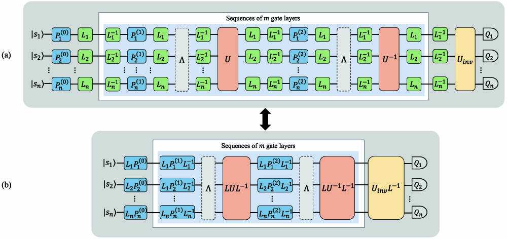
    Fig. 2. Illustrations of the noisy CCB circuit with local gauge transformation. For simplicity, we show the case that the local gates are noiseless. The grey dashed boxes denote the noise channel Λ. The orange boxes represent the target gate U and its inverse gate U1. The blue boxes represent the random Pauli gates. The green boxes represent the inserted local gates L and L1, where L=i=1nLi. The yellow box denotes the inverse gate for the m inner gate layers in the light blue boxes. In practice, we implement gates in circuit (b) while absorbing local gates L and L1 into twirling and target gates. Here, the target gate following gauge transformation becomes LUL1. Note that circuit (a) is equivalent to a CCB circuit with target gate U and noise channel 1Λ. Thus, it can be implemented to estimate Fccb(1Λ), which is close to F(Λ).
    Simulation results for the controlled-(TX) gate with eight different noise channels, each containing a N(μ,σ)-Pauli channel, an amplitude damping channel, and a correlation channel. The parameters for the amplitude damping channels and correlation channels are set to be the same for the eight channels. For the Pauli channel, the error parameters are set to {(μ,σ)} = {(0.995, 0.001), (0.990, 0.002), (0.980, 0.003), (0.970, 0.004), (0.960, 0.005), (0.950, 0.006), (0.940, 0.007), (0.930, 0.008)}. (a) The fidelity estimations with different error rates in 40 independent simulations. The green dashed line represents the theoretical fidelities. The two insert scatter plots show the fluctuations of estimated fidelities over different simulations. (b) Take the fifth simulation with a process fidelity of 95.98% as an example. The fitting curves of Eq. (10) for Qk=IZ,ZI,ZZ. The decay parameters derived from the curves are λIZ=0.9580, λZI=0.9550, λZZ=0.9577.
    Fig. 3. Simulation results for the controlled-(TX) gate with eight different noise channels, each containing a N(μ,σ)-Pauli channel, an amplitude damping channel, and a correlation channel. The parameters for the amplitude damping channels and correlation channels are set to be the same for the eight channels. For the Pauli channel, the error parameters are set to {(μ,σ)} = {(0.995, 0.001), (0.990, 0.002), (0.980, 0.003), (0.970, 0.004), (0.960, 0.005), (0.950, 0.006), (0.940, 0.007), (0.930, 0.008)}. (a) The fidelity estimations with different error rates in 40 independent simulations. The green dashed line represents the theoretical fidelities. The two insert scatter plots show the fluctuations of estimated fidelities over different simulations. (b) Take the fifth simulation with a process fidelity of 95.98% as an example. The fitting curves of Eq. (10) for Qk=IZ,ZI,ZZ. The decay parameters derived from the curves are λIZ=0.9580,  λZI=0.9550,  λZZ=0.9577.
    Simulation results for the five-qubit quantum error correcting encoding circuit with a noise channel composed of a depolarizing channel Λdep(ρ)=pρ+(1−p)I/d, where p=0.98, an amplitute damping channel, and a correlation channel. The theoretical process fidelity is F=94.70%. (a) Box plot of the CAB fidelities versus sampling number K with 40 independent simulations. The red boxes represent the distributions of the CAB fidelity estimations with respect to K. The orange points represent the distributions of CAB fidelities. (b) Box plots of the CAB and XEB fidelities versus K with 40 independent simulations. The green dashed line represents the theoretical process fidelity. The plots of CAB in (a) and (b) are the same with different scaling.
    Fig. 4. Simulation results for the five-qubit quantum error correcting encoding circuit with a noise channel composed of a depolarizing channel Λdep(ρ)=pρ+(1p)I/d, where p=0.98, an amplitute damping channel, and a correlation channel. The theoretical process fidelity is F=94.70%. (a) Box plot of the CAB fidelities versus sampling number K with 40 independent simulations. The red boxes represent the distributions of the CAB fidelity estimations with respect to K. The orange points represent the distributions of CAB fidelities. (b) Box plots of the CAB and XEB fidelities versus K with 40 independent simulations. The green dashed line represents the theoretical process fidelity. The plots of CAB in (a) and (b) are the same with different scaling.
    Illustrations of the CCB circuit with local gauge transformation. Circuit (a) is equivalent to the original CCB circuit in the main text if all of gates are ideal. The orange boxes represent the target gate U and its inverse gate U−1. The blue boxes represent the random Pauli gates. The green boxes represent the inserted local gates L and L−1, where L=⊗i=1nLi. The yellow box denote the inverse gate for the m inner gate layers in the light blue box. In practice, we implement gates in circuit (b) while absorbing local gates L and L−1 into twirling and target gates. Here, the target gate after gauge transformation becomes LUL−1.
    Fig. 5. Illustrations of the CCB circuit with local gauge transformation. Circuit (a) is equivalent to the original CCB circuit in the main text if all of gates are ideal. The orange boxes represent the target gate U and its inverse gate U1. The blue boxes represent the random Pauli gates. The green boxes represent the inserted local gates L and L1, where L=i=1nLi. The yellow box denote the inverse gate for the m inner gate layers in the light blue box. In practice, we implement gates in circuit (b) while absorbing local gates L and L1 into twirling and target gates. Here, the target gate after gauge transformation becomes LUL1.
    Five-qubit stabilizer encoding circuit.
    Fig. 6. Five-qubit stabilizer encoding circuit.
    Simulation results of CAB and ICRB for benchmarking a CZ gate. (a) The error bar of the fidelity obtained from 50 experiments via CAB and ICRB protocols. The x-axis represents the amount of single-shot measurements, and the y-axis represents the fidelity. The term “shot" represents the number of single shots associated with one sample sequence. One can see that CAB and ICRB can both obtain an accurate estimation of the process fidelity of a CZ gate. (b) The standard deviation of the fidelity obtained from 50 experiments via CAB and ICRB protocols. The x-axis represents the amount of single-shot measurements, and the y-axis represents the standard deviation of the fidelity. The figure shows that CAB has an advantage over ICRB with regard to standard deviation.
    Fig. 7. Simulation results of CAB and ICRB for benchmarking a CZ gate. (a) The error bar of the fidelity obtained from 50 experiments via CAB and ICRB protocols. The x-axis represents the amount of single-shot measurements, and the y-axis represents the fidelity. The term “shot" represents the number of single shots associated with one sample sequence. One can see that CAB and ICRB can both obtain an accurate estimation of the process fidelity of a CZ gate. (b) The standard deviation of the fidelity obtained from 50 experiments via CAB and ICRB protocols. The x-axis represents the amount of single-shot measurements, and the y-axis represents the standard deviation of the fidelity. The figure shows that CAB has an advantage over ICRB with regard to standard deviation.
    Yihong Zhang, Wenjun Yu, Pei Zeng, Guoding Liu, Xiongfeng Ma. Scalable fast benchmarking for individual quantum gates with local twirling[J]. Photonics Research, 2023, 11(1): 81
    Download Citation