Characterizing a quantum process has great importance in both the fundamental study and practical application of quantum information science. With the recent advent of noisy intermediate-scale quantum computing [1], benchmarking of quantum operations is critical for quantum control [2,3] as it provides an indicator for assessing experimental devices. Furthermore, it is essential for the development of high-precision quantum information processing instruments. Accurate benchmarking can reliably characterize the noise levels of quantum operations, and it plays a critical role in promoting fault-tolerant universal quantum computing [4,5]. In practice, we must evaluate the performance of a quantum circuit to verify whether a quantum algorithm or an error-correcting code is properly implemented in a quantum system.

Numerous approaches have been proposed to characterize quantum processes. Conventional methods such as quantum process tomography [6] provide a full description of a channel. However, these methods are impractical for large-scale quantum systems as the required experimental resources increase exponentially with the number of qubits, even with state-of-the-art techniques such as compressed sensing [7,8]. Direct fidelity estimation [9] tackles the scaling problem and characterizes the quantum process in terms of average fidelity. Unfortunately, the result inevitably contains extra errors from the state preparation and measurement (SPAM) and hence often over-estimates the noise levels. In reality, SPAM errors usually grow rapidly with the system size so that it is hard to characterize the quantum process accurately for large-scale quantum systems with direct fidelity estimation.

Randomized benchmarking (RB) and its variants have been proposed to avoid simultaneously the scaling problem and SPAM errors [10–16]. Standard RB estimates the average error rate of a specific gate set under the assumption of gate-independent or weakly-dependent noise. The gate set is normally selected to be the Clifford group and has been widely implemented in experiments [17–24]. Otherwise, to characterize a specific Clifford gate, a variant called interleaved RB was proposed. It utilizes random Clifford gates interleaved with the target gate [25]. The random gates here are considered to be the twirling gates for reference, whose fidelity should be measured separately to infer the fidelity of the target gate. The interleaved RB method is efficient and scalable in principle. However, it suffers from two severe problems in practice. The first is the compiling overhead for twirling operations. In reality, any operation needs to be compiled to one- and two-qubit gates native to the quantum system. Note that twirling gates are randomly picked from a gate set, like the Clifford group. In general, the average number of native gates used for compiling a single sample grows dramatically with the system size. The second is the gate-dependent noises introduced by twirling gates. Note that different twirling operations in a gate group can vary a lot in the depths of compiled circuits. For example, a local operation such as a Pauli gate can be implemented by a single layer circuit, while a complex entangling operation requires a deep circuit with massive native gates. The strong gate-dependent noises caused by the uneven compilations may bring inaccuracy to the fidelity estimation [26,27]. Consequently, the compiling overhead and gate-dependent noises introduced by twirling gates limit the scalability of the RB method in experiments.

Recently, there have been several variants of RB attempting to address the two compiling problems. For example, character benchmarking employs the character theory so that the quality parameters can be extracted from the local twirling operations [28]. Unfortunately, for the gate groups with an exponentially increasing number of quality parameters, this method requires an exponential amount of SPAM settings. Besides, character benchmarking is still caught in the aforementioned compiling problems for the final inverse gate and can be hardly applied for a generic multi-qubit quantum operation. Another inspiring attempt called cycle benchmarking aims to estimate the fidelity of the target gate by interleaving it with the Pauli gate set. However, it is restricted to the Clifford gates [29]. In addition, cycle benchmarking requires numerous repetitions for the gates with large cyclic numbers, which is common for multi-qubit gates. Hence, this method cannot efficiently benchmark a wide class of gates. The cross-entropy benchmarking (XEB) characterizes the fidelity of a generic quantum gate reflected by linear cross-entropy using local Clifford gate twirling [30]. However, the Haar measure assumption in XEB may lead to poor fidelity estimation when the size of the target gate is large. Thus, how to efficiently and reliably estimate the fidelity of a large-scale quantum process from a universal gate set remains an open problem.

This work proposes two scalable and efficient protocols to tackle the compiling problems as well as the SPAM error issues simultaneously, which we label character-cycle benchmarking (CCB) and character-average benchmarking (CAB), respectively. The protocols utilize local twirling to reliably characterize the fidelity of an individual multi-qubit quantum operation. We employ the Pauli and the local Clifford gates for twirling and extend the applicable gate set to non-Clifford gates via the local gauge transformation. The efficiency and reliability of the protocols are shown by rigorous mathematical derivations and by numerical simulations under realistic physical assumptions.

Let us denote the quantum operation of a unitary matrix U acting on an n-qubit quantum state, ρ, by the calligraphic letter U, i.e., U(ρ)=UρU−1, and the noisy implementation by U˜. One can evaluate the quality of U˜ by the process fidelity of the noise channel Λ=U−1∘U˜, F(Λ)=1d2∑i=04n−1λi,(1)where λi=d−1Tr(PiΛ(Pi)) is the Pauli fidelity associated with the Pauli operator Pi∈Pn, and d=2n is the dimension of the quantum system. Here, Pn denotes the n-qubit Pauli group, containing the tensor product of the identity operation I and three Pauli matrices X,Y,Z.

In practice, it is costly to figure out all the parameters λ0,λ1,⋯,λ4n−1 as their number increases exponentially with n. Instead, one can estimate the process fidelity via repeatable sampling of λ0,λ1,⋯,λ4n−1. Concretely, one samples a sufficient number of Pauli operators {Pj} and averages the corresponding {λj}, F(Λ)≈1MΣ{Pj}λj,(2)where M is the number of samples and the summation takes over the sample set.

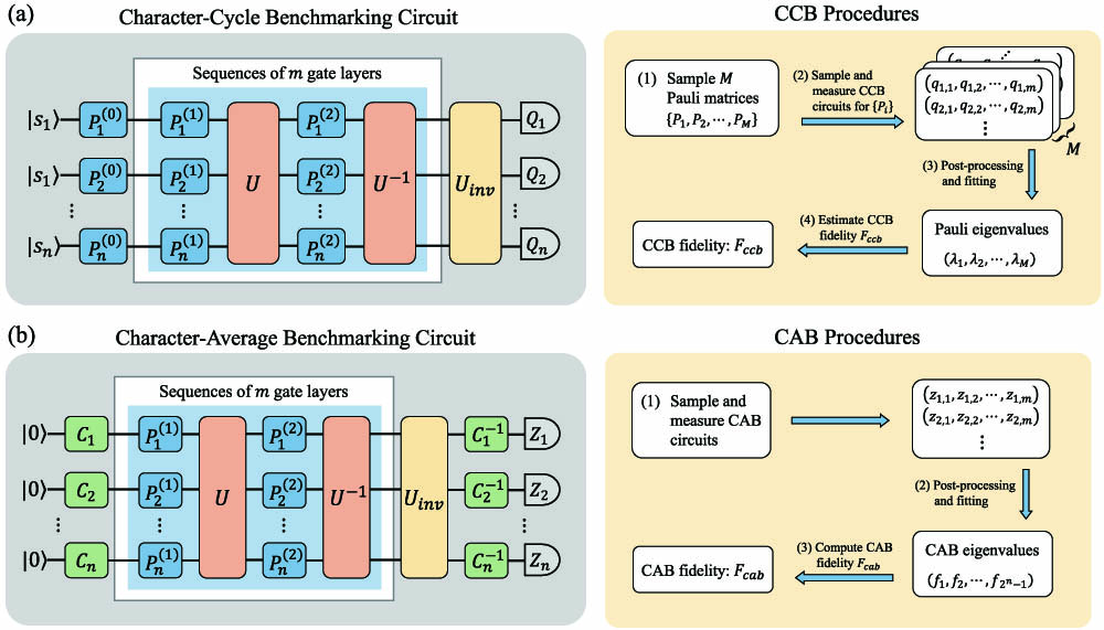
Here, we propose a CCB protocol that employs the key techniques of the cycle [29] and character benchmarking [28]. Specifically, we extract different Pauli fidelities through applying specific initial states and measurements and utilize the character theory to fully separate the SPAM errors. The schematic circuit of the CCB protocol is shown in Fig. 1(a). Let us start with the Clifford case, where the target gate belongs to the n-qubit Clifford group Cn. The inner random gate layer consists of the target gate U and its inverse gate U−1, interleaved with two random Pauli gate layers. The Pauli gates are the reference gates employed to perform local Pauli twirling over the generic quantum noise channel Λ and turn it into ΛP=14nΣ{Pj∈Pn}Pj−1∘Λ∘Pj,(3)where Λ contains the errors of Pauli gates and target gate U; ΛP is a Pauli channel satisfying ΛP(ρ)=∑jpjPjρPj, and pj is the Pauli error rate related to Pj.

Note that the introduction of the inverse target gate U−1 is the major difference between CCB and cycle benchmarking. In cycle benchmarking, we need to repeat U for multiples of l times, where l is the cyclic number of U, i.e., Ul=I. In general, l can be quite large for a wide class of Clifford gates, which is prohibitive for the experiments. For example, the five-qubit quantum error-correcting encoding circuit requires l=124. The CCB protocol improves the efficiency and application scope via substituting a single U−1 for multiple repetitions of U in cycle benchmarking. In many quantum platforms, such as superconducting quantum processors, the inverse gates of the native gates are also native. Typical examples include single-qubit gates, CZ, and iSWAP. Thus, the inverse gates of native gates are normally easy to implement. More generally, if U is composed of several native gates, the difficulty to implement U and U−1 is often the same. Based on this consideration, the introduction of U−1 does not increase the implementation difficulty of CCB in most cases.

In CCB, the randomization of Pauli gates in the inner gate layers will generate a composite channel U−1∘ΛP(−)∘U∘ΛP, where ΛP and ΛP(−) are the Pauli-twirled channels corresponding to gates U and U−1, respectively. Note that this composite channel is a Pauli channel for Clifford gate U. The fidelity we aim to estimate in the CCB protocol is defined as the CCB fidelity, Fccb=F(U−1∘ΛP(−)∘U∘ΛP),(4)which contains the fidelities of U and U−1. When the noise channel of U is the same as that of U−1, which is valid for most of the experimental platforms, the CCB fidelity is simplified as Fccb(Λ)=F(U−1∘ΛP∘U∘ΛP).(5)

Equation (5) is a lower bound of the process fidelity F(Λ) in terms of the expectation value, as proved in Appendix B.2. In the following context, we will employ Eq. (5) as our CCB fidelity metric model and our arguments apply to the general model of Eq. (4) as well. The difference between Fccb and F is normally small because the physical realizations of the qubits in one experimental platform are similar and the qualities of these qubits will not differ too much. Note that if ΛP is a depolarizing channel, then Fccb=F. Thus, the CCB fidelity can be seen as a reliable metric for the noise channel Λ.

The procedure of the CCB protocol is as follows. 1.Sample a Pauli operator Pj and initialize state |s⟩ such that Pj|s⟩=|s⟩.2.Apply a gate sequence Sccb composed of a Pauli gate P(0), m inner gate layers denoted by Sm, and inverse gate Sm−1.3.Perform measurement Pj and then calculate the Pj-weighted survival probability fj(m,Sccb)=χj(P(0))·Tr(PjSccb(ρs)), where χj(P(0))=1 if Pj commutes with P(0) and −1 otherwise.4.Repeat steps (2) and (3) for several times for different m and fit the Pj-weighted fidelity to f^j(m)=Ajλj2m.5.Repeat steps (1)–(4) for several times and finally estimate the CCB fidelity as Fccb=avejλj.

Here, the estimated fidelity Fccb includes the errors from the local reference gate set Pn. To remove these extra errors, one can employ the interleaved RB technique, by performing additional CCB with a target gate of identity I to estimate the reference fidelity FccbI. Then, one can infer the fidelity of the target gate as Fccb/FccbI. In practice, the errors of local gates are often negligible, and hence, we focus on Fccb in the following discussions.

Note that our inverse gate Sm−1 is a Pauli gate and thus will not introduce extra gate compiling overhead. In contrast, character benchmarking for a single multi-qubit Clifford gate [28] requires a global inverse gate and a complicated compiling process. This may cause strong gate-dependent errors and lead to inaccuracy for fidelity estimation, especially for multi-qubit quantum operations. The CCB protocol maintains the local structure of reference and inverse gates and thus avoids the compiling problems.

In the CCB protocol, one needs to average Pauli fidelities λj to estimate Fccb. The sampling complexity for the CCB protocol is given by the following theorem.

Theorem 1 (informal version). For ann-qubit quantum noise channel, to estimate the CCB fidelity within the confidence interval[F^ccb−ϵM−ϵb,F^ccb+ϵM+ϵb]with probability greater than1−δ, one needs to sampleMPauli fidelities where each Pauli fidelity is estimated viaKrandom sequences. The confidence probability of the estimation is given by Pr(|F^ccb−F¯ccb|≤ϵM+ϵb)≥1−δ,(6)where ϵM≤O(−logδM) and ϵb≤O(K−1)+O((−logδK)3/2).

Here, the total number of samples, or sample complexity, depends on M and K. If the number of random sequences for each Pauli fidelity is the same, then the sample complexity is simply given by MK. Theorem 1 shows that the sample complexity only depends on fidelity precision ϵM,ϵb, and confidence level δ. The independence on system size n reflects the strong scalability of the CCB protocol. A more detailed description of the result is shown in Theorem 2.

Now, let us extend the applicable gates for the CCB protocol to non-Clifford gates. One can introduce local gauge transformation L to the twirling gate set, Pn→LPnL−1, where L is an arbitrary local unitary operation L∈U(2)⊗n. Note that the transformed twirling gate set LPnL−1 is still local. Then, we can show that the applicable target gate set becomes LCnL−1, where Cn is the n-qubit Clifford gate set.

To benchmark a gate LUL−1 from gate group LCnL−1, we insert local gates L and L−1 between the twirling gates and the target gates in the original CCB circuit, as shown in Fig. 2(a). Here, L=⊗i=1nLi, where Li can be an arbitrary single-qubit gate. In practice, the local gates are absorbed into twirling gates and target gates and do not need to be implemented individually as manifested in Fig. 2(b). The character gate LP(0) and the twirling gate LP(1)L−1 will be merged into a single gate in implementation as well. Details of the derivation are shown in Appendix B.3.

As shown in Fig. 2, the CCB circuit with local gauge transformation L and noise channel Λ is equivalent to the original CCB circuit with noise channel L−1ΛL. Thus, one can obtain Fccb(L−1ΛL), which is close to the process fidelity F(L−1ΛL). As process fidelity is gauge-invariant, that is, F(L−1ΛL)=F(Λ), one can estimate the process fidelity of Λ as the performance indicator of gate LUL−1.

Now, let us check out what kinds of quantum gates belong to the set S={LUL−1|L∈U(2)⊗n,U∈Cn}.

First, notice that if a unitary U∈S, then for any L∈U(2)⊗n, LUL−1∈S. As any unitary is generated by a Hamiltonian, that is U=eiH where H is Hermitian, one can conclude that if eiH∈S, then for any L∈U(2)⊗n, LeiHL−1=eiLHL−1∈S.

Take a step forward. If a controlled-eiH∈S, then through local gauge transformation I⊗L, (I⊗L)controlled−eiH(I⊗L)−1=controlled−eiLHL−1∈S. The arguments also apply to the case of multi-controlled gates.

The two observations inspire us to first represent Clifford gates in the form of eiH or multiple controlled-eiH, then replace H with LHL−1 to find other gates in S. Take CZ as an example. CZ=eiπ|11⟩⟨11|= controlled-e−iπ2Z. Through local gauge transformation, one can transform |11⟩ to any product state |ψϕ⟩ and transform e−iπ2Z to any π-rotation e−iπ2σ→·θ→, where σ→=(X,Y,Z) and θ→ is a unit vector. Thus, for any two-qubit product state |ψϕ⟩, we have e−iπ|ψϕ⟩⟨ψϕ|∈S. In addition, any controlled-π rotation, such as controlled-H and controlled-TX, belongs to S.

Reversely, controlled-S= controlled-e−iπ4Z is a controlled-π2 rotation. As any controlled-π2 rotation is not Clifford, one can conclude that controlled-S does not belong to S. Similarly, Tofolli = controlled-controlled-e−iπ2X is a controlled-controlled-π rotation. As any controlled-controlled-π rotation is not Clifford, one can conclude that Tofolli does not belong to S either. It is interesting to decide whether a quantum gate belongs to S in a more general case, and we leave it for future work.

We can take the CCB protocol one step further. Observe that in CCB, one needs to implement the fitting procedures for each sampled Pauli operator Pj to estimate Pauli fidelity λj. Each estimation requires specific initial state, measurement, and independent randomization procedures. We can further simplify these procedures by introducing the local Clifford group C1⊗n. Recall that in a qubit system, the Clifford twirling depolarizes a channel via averaging the error rates in X,Y,Z bases [13]. Then for an n-qubit system, the twirling over C1⊗n would partially depolarize a channel and average out 4n Pauli fidelities λj into 2n terms. These 2n values can be obtained from the Z⊗n basis measurement only with additional data post-processing.

Based on the local Clifford twirling, we propose the CAB protocol as an improvement of the CCB protocol. The schematic circuit of CAB is shown in Fig. 1(b), with the detailed procedures described in Box 1. Like the CCB protocol, we can extend the target gate set beyond the Clifford group by employing local gauge transformation. Here, to suppress statistical fluctuations, we remove the character technique. Detailed description and analysis of the CCB and CAB protocols are presented in Appendix B.

Similar to the CCB protocol, the randomization over m gate layers inside the blue box in Fig. 1(b) will generate a Pauli channel ΛP(m)=(U−1∘ΛP∘U∘ΛP)m. The local Clifford gates in the beginning and end of the circuit jointly perform local unitary 2-design twirling, which transforms the Pauli channel ΛP(m) into a partially depolarizing channel ΛC(m). Here, the quantum channel ΛC(m) contains less independent parameters than the original ΛP(m). It holds the unique value of fidelity for every disjoint Pauli subset in Rn={{I},{X,Y,Z}}⊗n. The Pauli fidelities in ΛC(m) can be seen as the average values of those in ΛP(m), μk2m=∑Pj∈σkλj2m/|σk|, where {λj2m} are the Pauli fidelities of the channel ΛP(m). The local Clifford twirling here averages multi exponential decays into one exponential decay and captures all the information of the noise channel, as shown in Eq. (11). The comparison between Fcab and Fccb is shown in Lemma 3 in Appendix B.5, while the CCB protocol employs a sampling method as in Eq. (2), which only contains partial information of the noise channel. Thus, one can intuitively conclude that the CAB protocol is more efficient than the CCB protocol, as demonstrated in later simulations.

In numerical simulations, we characterize a two-qubit controlled-(TX) gate and a five-qubit quantum error correcting encoding circuit, respectively. Furthermore, we simulate the noise channel for the target gate with a realistic error model that contains a Pauli channel, an amplitude damping channel, and a correlation channel. In the simulation, the Pauli fidelities of the Pauli channel are randomly sampled from a normal distribution N(μ,σ), which we call the N(μ,σ)-Pauli channel. Here, the error parameter μ reflects the quality of the Pauli channel and σ implies the discrepancy of the channel, i.e., the differences among Pauli fidelities. The detailed descriptions for the error models and simulations are presented in Appendix D.

For the controlled-(TX) gate, we take (I⊗T)·Pn(I⊗T−1) as the twirling gate set, where T is the π/8-phase gate, T=exp(−iπZ/8), and I⊗T is the local gauge transformation. We simulate the CAB and CCB protocols on the controlled-(TX) gate with 8 different noise channels. For each noise channel, we take 40 independent simulations for both CAB and CCB protocols. In CCB simulations, we sample M=10 Pauli operators to estimate Fccb.

Figure 3(a) shows Fcab and Fccb versus the error rate r=1−F for the controlled-(TX) gate with different noise channels. We observe that when the standard deviation of error parameters σ grows, the error bars of Fcab and Fccb become larger. Intuitively, the discrepancy of the Pauli fidelities is one of the key reasons for the fluctuations of Fcab and Fccb. The fluctuations for the estimations will reach the minimum level when the noise channel is completely depolarizing. Besides, the error bar of CAB is smaller than the error bar of CCB. This shows that under the same estimation accuracy, the sampling complexity, i.e., the amount of sampling sequences in total, of the CAB protocol is smaller than that of the CCB protocol, especially when the discrepancy of the noise channel is large. In Fig. 3(b), we take one of the eight noise channels as an example and show the three fitting curves of Eq. (10) for the CAB protocol. The resulting CAB fidelity is Fcab=95.99%, which is very close to the theoretical value of process fidelity F=95.98%.

For the five-qubit error correcting encoding circuit, which is a Clifford gate, we take the Pauli group Pn as the twirling gate set. For the simplicity of simulation, we set the Pauli channel to be a depolarizing channel Λdep(ρ)=pρ+(1−p)I/d where p=0.98. The setting of the amplitude damping and correlation channels remains the same. Furthermore, we simulate the CAB and XEB protocols to characterize the noisy five-qubit encoding circuit. For each protocol, we run 40 independent simulations. In each simulation, we take the sampling number of gate sequences as K=50,⋯,500 for each sequence length m. The box plot of Fcab versus K is shown in Fig. 4(a). We can see that when K grows, the fluctuations of Fcab become smaller. When K is not too large, like K=50, the fluctuation is already small enough, which implies that the CAB protocol works well with few sampling sequences needed.

In Fig. 4(b), we show the box plots of Fcab and XEB fidelities Fxeb versus the sampling number K. It is clear to see that compared with Fxeb, Fcab is much closer to the theoretical process fidelity F=94.7%. Meanwhile, the convergence of Fcab is much better than that of Fxeb. This implies that the required K for CAB is much smaller than that of XEB under the same estimation accuracy.

To give a concrete example, we take 20 CAB simulations and 20 XEB simulations under the same noise channel. From the simulation results, we find that for CAB, when Kcab=20, the standard deviation over the 20 simulations is σcab=3.25×10−4, while for XEB, when Kxeb=20,000, the standard deviation is σxeb=4.29×10−4. This shows that to estimate the fidelities with standard deviations around 4×10−4, the required Kxeb is over 1000 times larger than Kcab. Thus, we can conclude that the performance of CAB protocol is three orders of magnitude better than that of XEB protocol in terms of the sampling complexity.

The simulation results reveal the strong scalability and reliability of our protocols, especially the CAB protocol. The fluctuation of estimated CAB fidelity is small even for multi-qubit gates. We believe the CAB protocols can provide fast feedback in experimental designs and promote the development of universal fault-tolerant quantum computing.

The characterization of large-scale individual quantum processes is crucial to the development of near-term quantum devices. However, to the best of our knowledge, there are no scalable and practical methods as of yet that could benchmark multi-qubit universal gate-set currently. In this work, we propose and demonstrate efficient and scalable randomized benchmarking protocols—CCB and CAB that can individually characterize a wide class of quantum gates including and beyond the Clifford set. The key technique of our protocols is using the local reference gate-set for twirling, which avoid the inaccuracy of the estimation caused by gate-compiling overhead and gate-dependent noises. The method of local gauge transformation offers a tool for characterizing non-Clifford gates. The sampling and measurement complexity are independent of the qubit number of gate, which means our benchmarking protocols can be generalized to large-scale quantum systems.

Our protocols maintain the simplicity and robustness of the conventional RB method, and estimate the quantity of most interest—process fidelity of the target gates. We believe our protocols will promote the development of universal fault-tolerant quantum computing. Furthermore, it would also be interesting to extend our randomization and estimation methods for characterizing other properties such as unitarity and coherence, which we leave for future research.

Acknowledgment. We acknowledge B. Chen for the insightful discussions.